PS. Here is a hypothesis of why is more visible in @d_fens capture.
If the pattern is inherent/related to the sensor, it would be similar in both captures (with/without sharpness/denoise/jpg), but it is significantly less on the captures.
The illuminant+sensor has inherent noise. If the noise combination is greater in one case than in the other, the smoothing of the processing (denoise/sharpness/compression) would make it less apparent. If the illuminant noise is greater, the smoothing of the processing would actually make it more visible.
In other words, if the noise amplitude is smaller than the pattern threshold (in the plot) while still there, it would be less visible.
Oh, that is very interesting. So it’s not libcamera, but the sensor which produces this pattern! And looking at the metadata of the capture (" 20231025test1.txt"), the digital gain is a solid 1.000.
One suspect I could come up with is what some users call the “Star Eater Algorithm” (more marketing style: “in-sensor defective pixel compensation” - a thing which is implemented right in the sensor (here’s a discussion of this topic). Not sure at the moment whether there is an option to turn this thing off in either libcamera-apps or via picamera2…
… ok, here’s an update on switching off “DCP”…
For libcamera-apps, in the software doc it is suggested:
libcamerauses open source drivers for all the image sensors, so the mechanism for enabling or disabling on-sensor DPC (Defective Pixel Correction) is different. The imx477 (HQ cam) driver enables on-sensor DPC by default; to disable it the user should, as root, enter
echo 0 > /sys/module/imx477/parameters/dpc_enable
And according to this recent issue, a similar strategy is required for picamera2:
The Linux kernel driver will let you disable this via a kernel module parameter. For the HQ cam, for example, do the following
sudo su # you will have to be root to change it
echo 0 > /sys/module/imx477/parameters/dpc_enable
So the next experiment would be to disable DPC completely and see whether this pattern is still there…
If it’s not available in the camera directly, you should be able to compensate for this in software, using the same technique used in astrophotography: for each set of images you shoot, you take a few dark and flat exposures, and those get stacked together into an average image. Darks are images taken with the lens cap on, to locate and compensate for amp glow in the sensor. And flats are images taken of a flat neutral grey (the technique most people use is putting a couple white t-shirts over the end of the telescope and taking images in daylight - though you can use a highly diffuse light source as well, as long as you know it’s flat).
Those are then used to locate any discrepancies in the sensor. This is basically a map of pixels and how much they need to be compensated for digitally to arrive at a completely flat image free of exposure variations. Once you know that, you can apply the same compensation to the exposed frame and the end result should be free of these patterns.
I am fairly certain scanners like the ScanStation do this as part of their camera calibration routines. While astrophoto people are a bit nutty about this and do it every night, I don’t believe it’s necessary to do it that frequently. The sensor map shouldn’t change that much over time, save for dead pixels or stuff like that.
Well, in another life, I worked with a special logarithmic image sensor where the individual pixels had a logarithmic response curve by design (that is different from the log-image you might get from an ARRI Alexa or so, where the pixels are still linear in response and the log is calculated afterwards). This logarithmic sensor required a different blacklevel and gain compensation for each individual pixel, and that compensation was also temperature-dependent. Once this worked (we implemented that in a FPGA), the dynamic range was fantastic for the purpose we used this chip - a single fixed f-stop could be used for moonlit scenes as well as for sun-flooded scenery.
The thing here is the following: modern sensors tend to have quite a bit of image processing internally. So what you are getting out of the sensor is nowadays strictly speaking not really “raw” data. To make things even more complicated, specifically the Star Eater algorithm is in its effect non-linear. So the standard approach you suggested would not work in this case (as it is intrinsically a linear operation). But it is fine for compensating @PM490’s or my dark spots (I wonder how @d_fens got his sensor array so clean ![]() )
)
the image with
echo 0 > /sys/module/imx477/parameters/dpc_enable
and
libcamera-still --gain 1.0 --shutter 50 --awbgains=1.58,1.86 --awb=daylight --tuning-file=/usr/share/libcamera/ipa/rpi/vc4/imx477_scientific.json --encoding png --denoise off --sharpness=0 --rawfull 1 --raw 1 --metadata dpc_disabled --output dpc_disabled.png
also shows this:
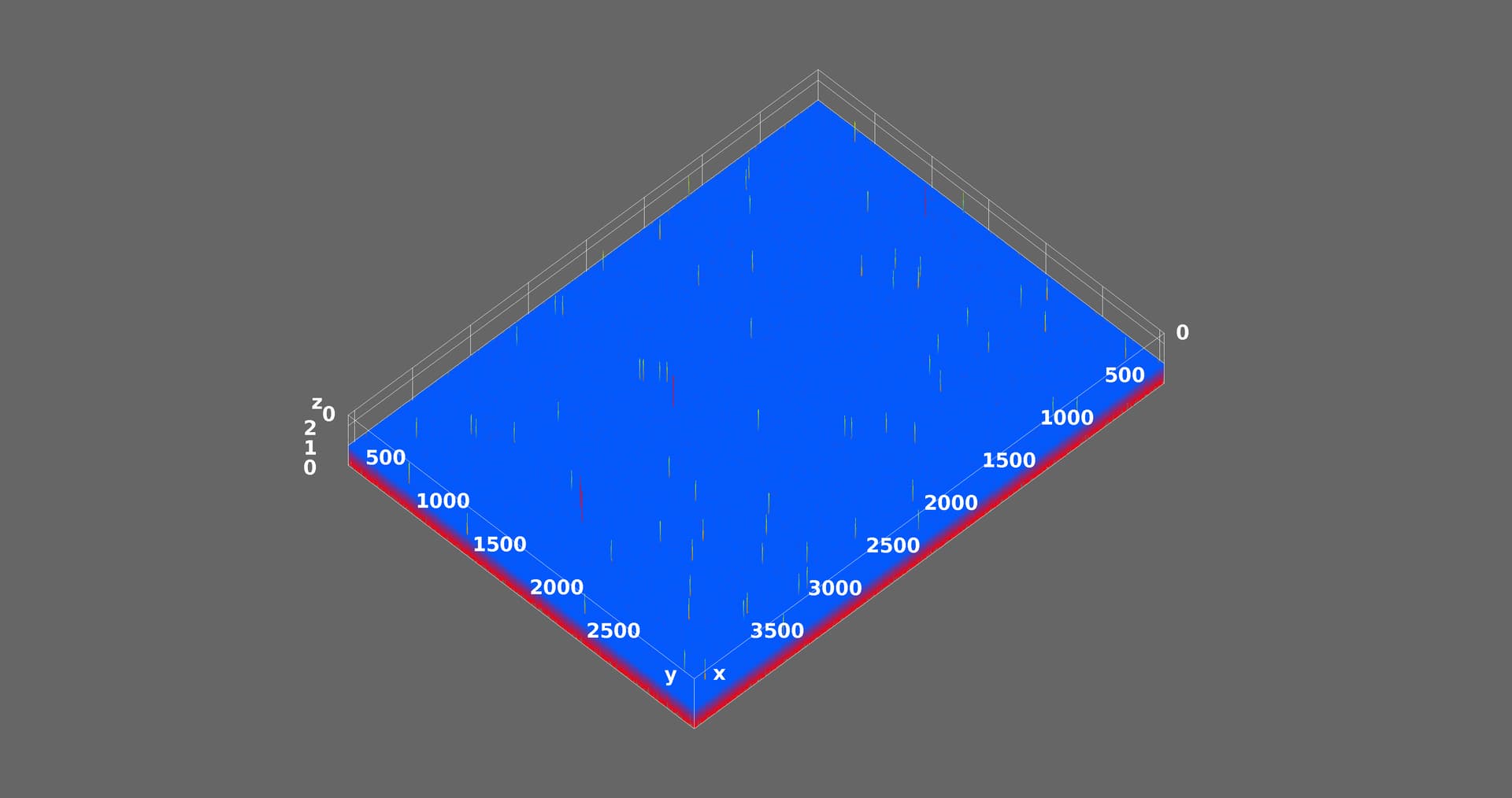
and regarding the dark spots: it’s just a question of perspective - topdown view shows the spots I still can’t get rid of:
Ok, so my world is again in balance ![]() It’s really hard to get the sensor clean!
It’s really hard to get the sensor clean!
Your result with DPC disabled is disappointing. This basically rules out DCP as a source for the observed pattern. Your and @PM490’s experiments seem to indicate that what the sensor delivers as raw data has already seen some processing directly in the sensor chip. Modern times! But: these variations you see are probably tiny with respect to the real image signal; especially within the context of the tiny formats we are aiming at, film grain will create a much stronger signal.
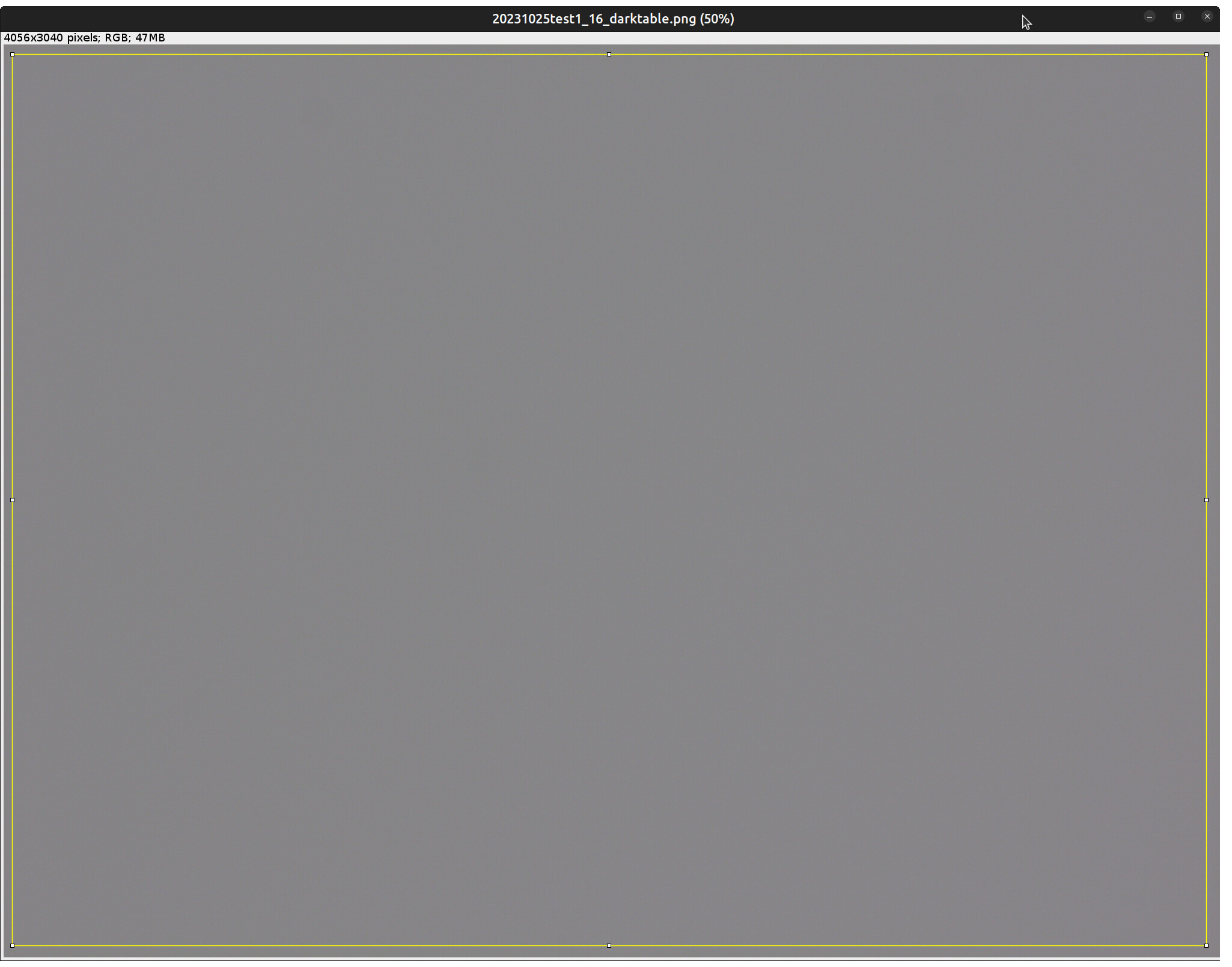
Plot from a DNG (converted to 16 bit png in Darktable) with the cap on.
As requested. Pattern still there.
Thanks for the experiment! So its not the “Star Eater algorithm”. To bad, would have been a simple explanation. At the moment, I have no good idea what we are looking at…
1 Like
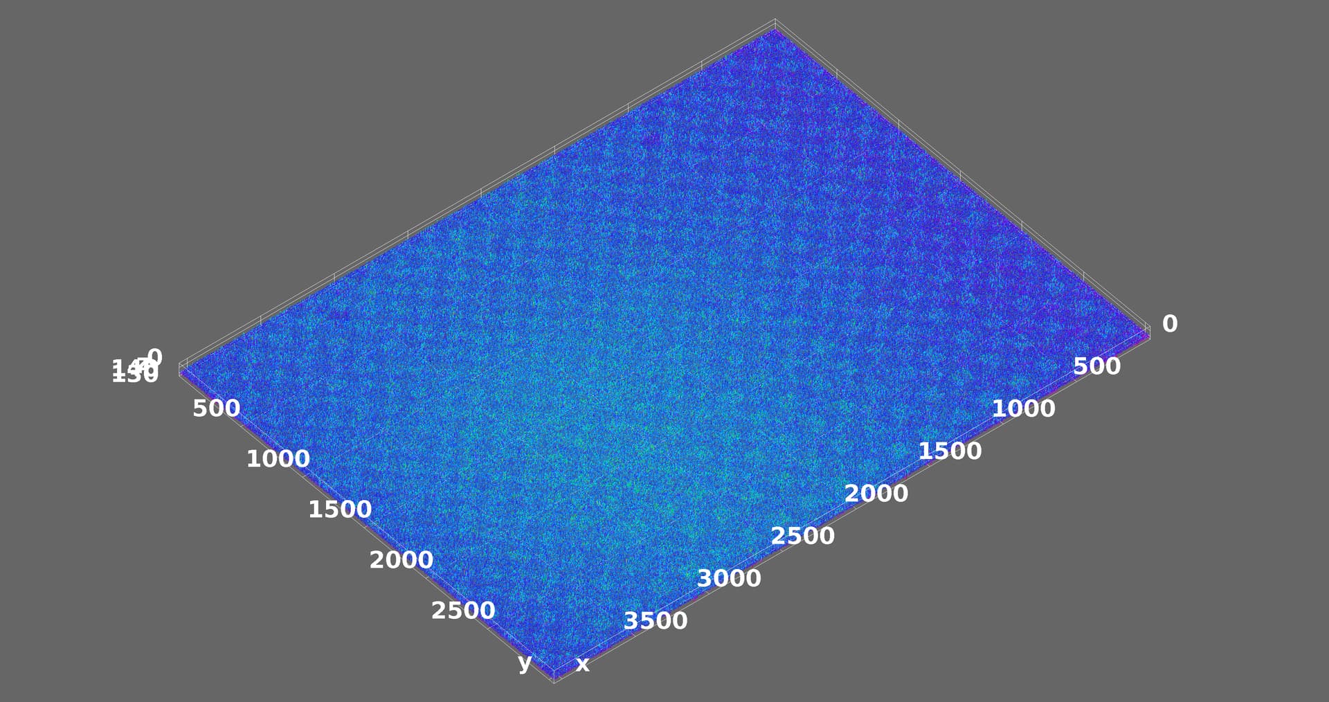
@PM490 - I did download your DNG-file and enhanced the contrast in RawTherapee, in order to examine the patterns more closely. Now, here’s the result:
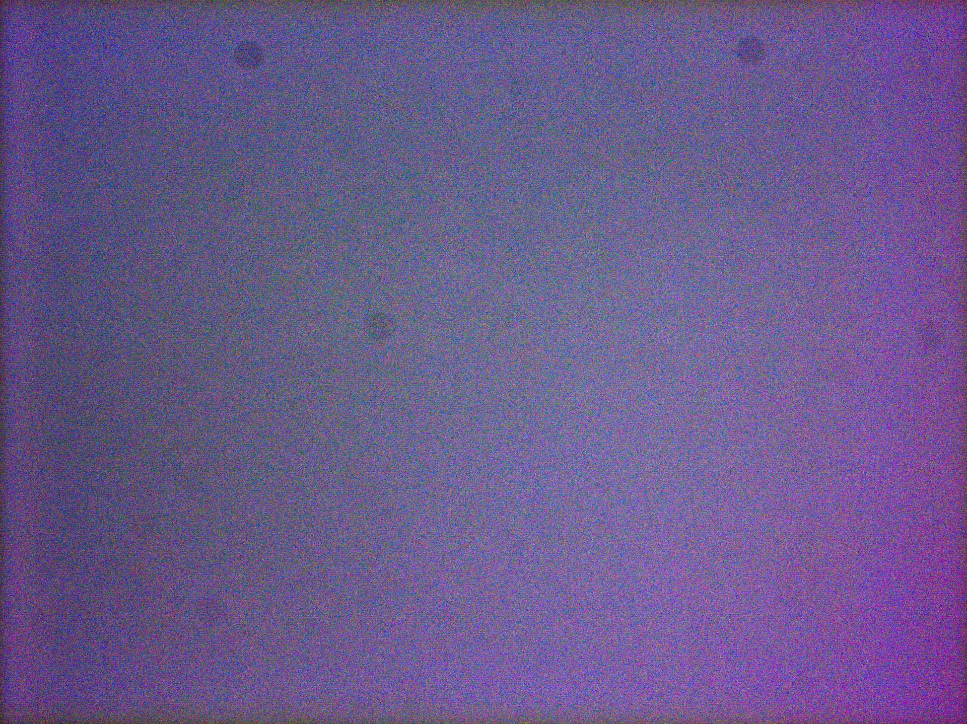
I do not notice any pattern of periodicity in this image.
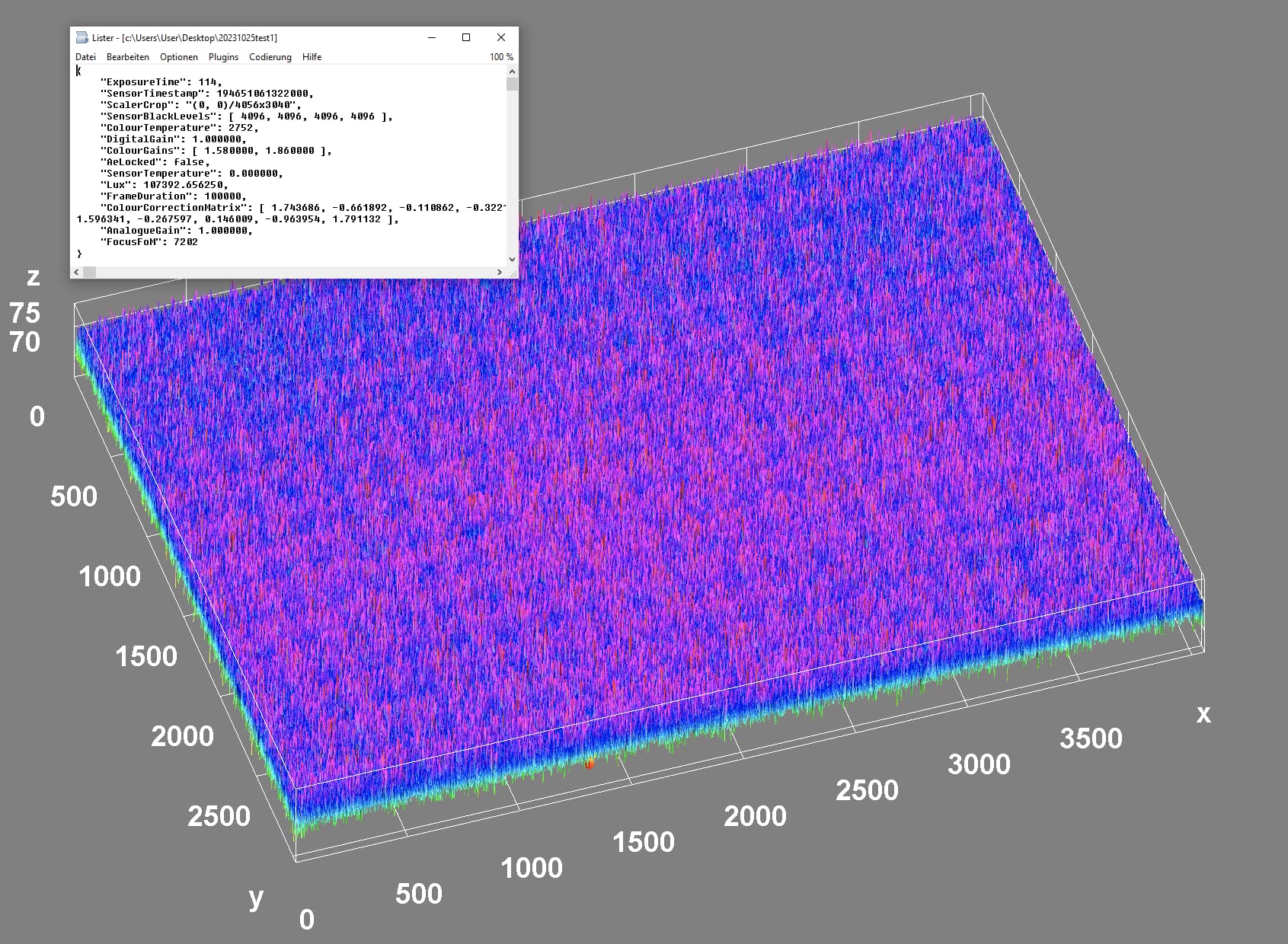
Compare this to the image @d_fens posted above:
where there are at least two patterns with different spatial frequency visible. One with rather bright horizontal and vertical lines, dividing the whole image area in a 8x6 patchwork, and a smaller pattern, composed from small noisy blobs.
Could the observed patterns be an artifact introduced by ImageJ? I would expect the patterns to show up at least a tiny bit in any sufficiently contrast-enhanced version…
By the way, the absence of any visible pattern is also true for a contrast-enhanced version of “20231025test1.jpg” - I assume, that is the actual .jpg captured.
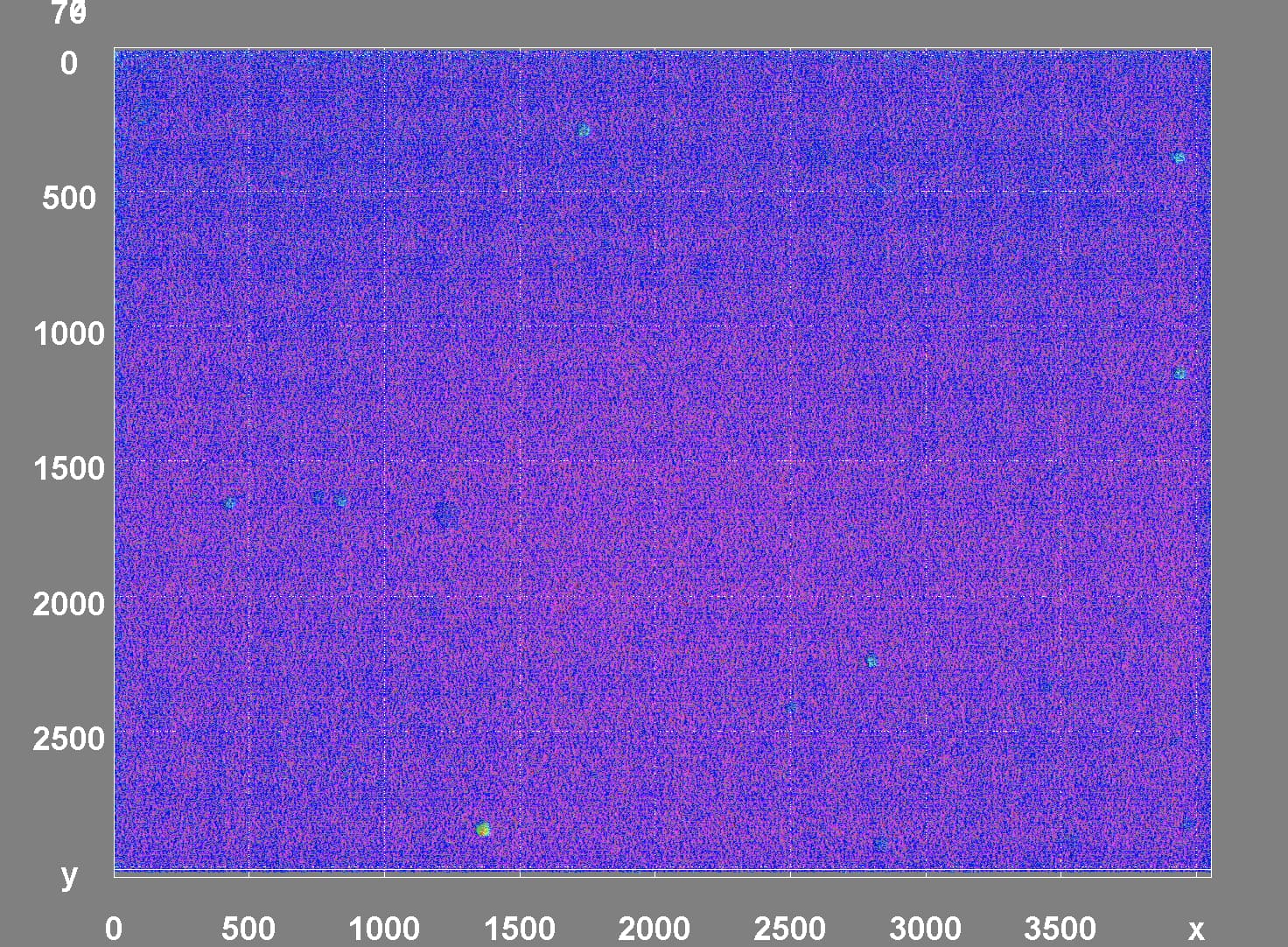
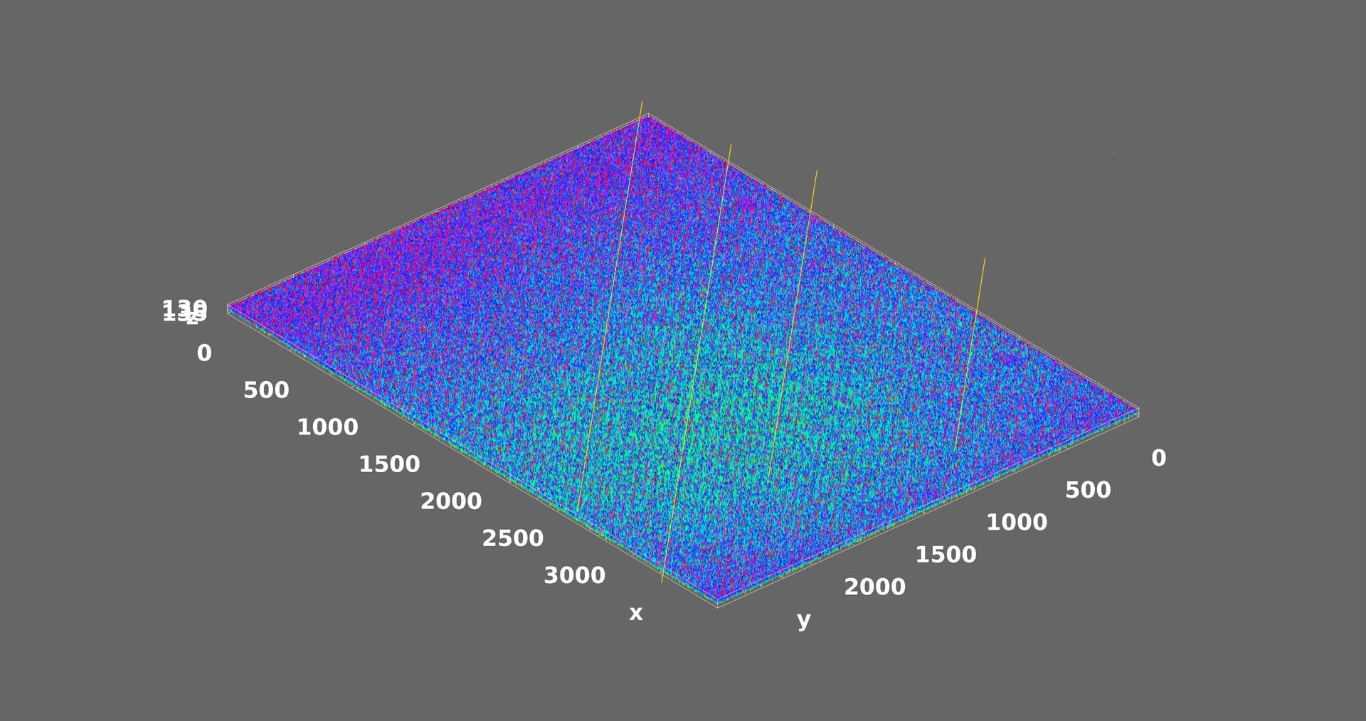
I was also wondering why the pattern was invisible in any other form. Here is a contrast enhance (in ImageJ) and a plot of a slice. The slice was selected because the area has the known visible spots.
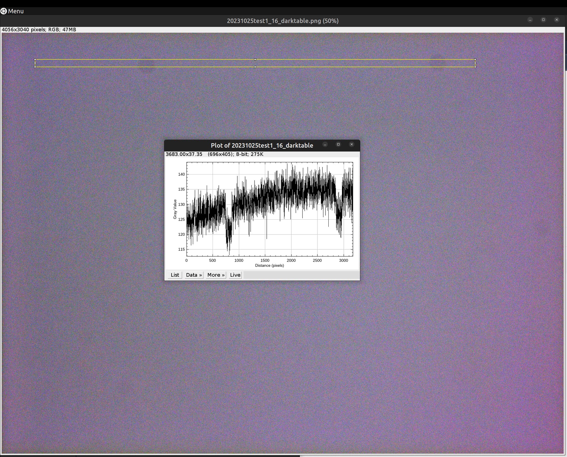
I think the spots should show in the bottom view perspective too, as these did on the previous plot.
In the absence of another explanation, since this is only visible in the 3D surface plot plug-in, it may be an artifact introduced by it. From the above slice, it does not show in other ImageJ areas.
Finally, the issue is analyzed ![]()
I contacted the author of the Plugin Professor Dr. Barthel and he was so kind and swiftly explained what’s actually happening here:
So thanks to his explanations we now can trust the HQ Camera, Sensor and libcamera2 pipeline again ![]()
3 Likes
these are the white grid lines of the 3D Grid shining through so that’s normal
well, provided the scientific tuning file is used… ![]()
1 Like
I think the hammer smashed a bug!
Actually not sure I agree with this explanation.
The pattern is most visible when looking at the plot from the bottom perspective. If instead of using the entire image, one selects a very large portion (almost the entire image), which would also have an unequal ratio to the grid size…
The bottom-view-tile-pattern artifact is no longer presented.

When the selection is removed, under the same surface plot parameters, the bottom-view-tile-pattern artifact is back.
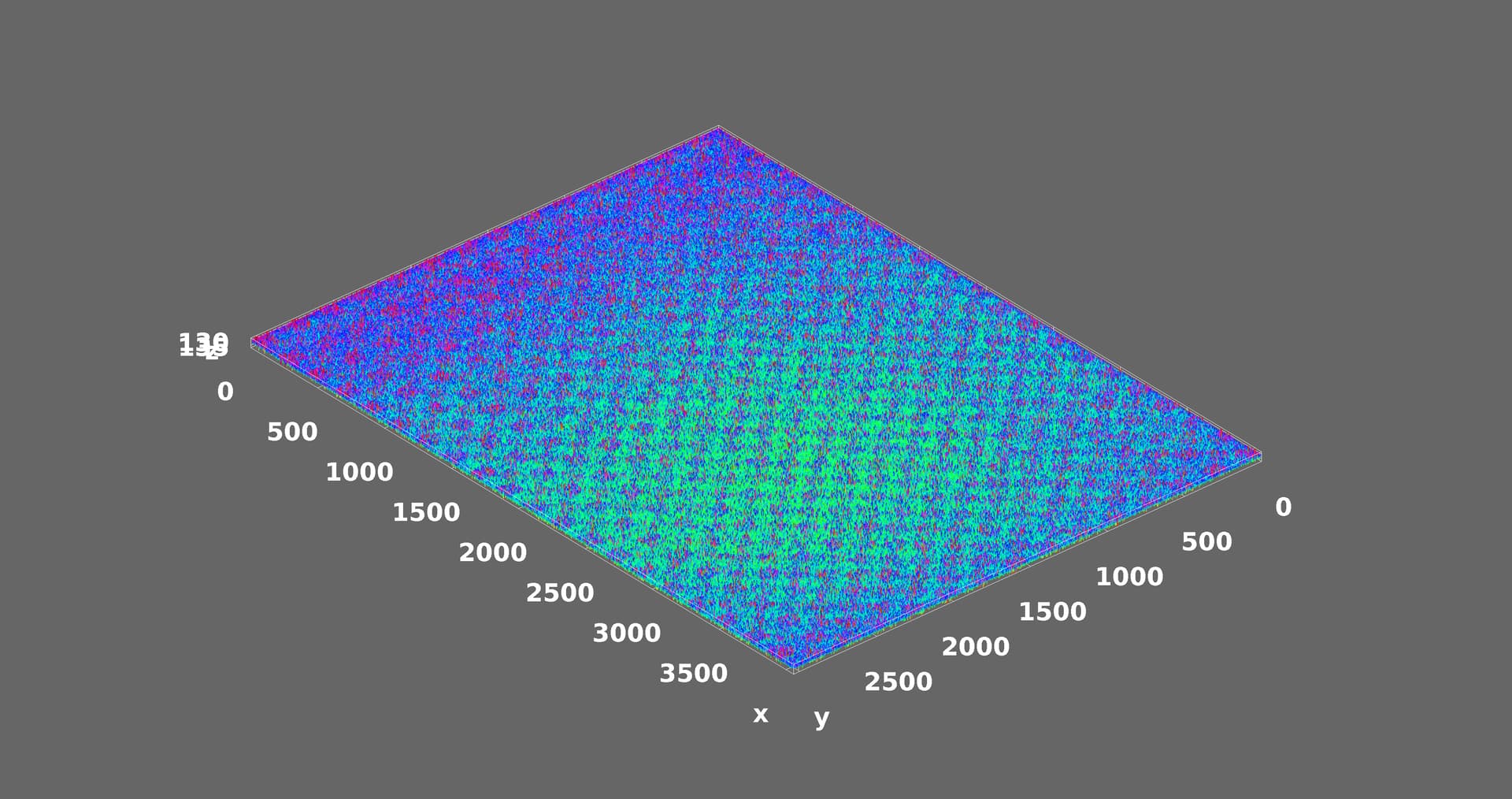
In all plots I produced, the grid was set to 1024.
@d_fens if you pass this info to Dr. Barthel, please convey my gratitude for creating the plug-in which has been very useful in our application.

from this angle, the high frequency pattern is best noted by the diagonal structure of the peaks i guess
[quote="PM490, post:34, topic:2470]
@d_fens if you pass this info to Dr. Barthel, please convey my gratitude for creating the plug-in which has been very useful in our application.
[/quote]
Yup, i’ll do that

I have turned to hacking a tool to see spots a bit better…
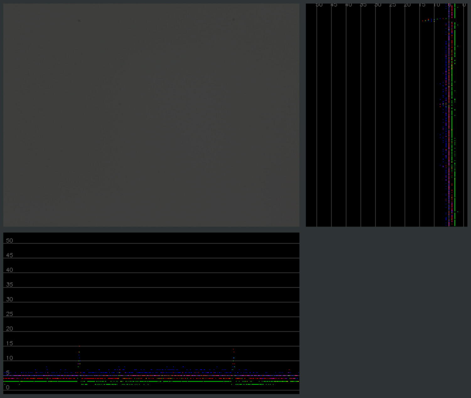
The chart is the maxVal-minVal for every column (bottom) and row (right) from the image (top/left).
When narrowing to a couple of x coordinates for columns and a couple of y coordinates for rows, no tile pattern was visible (not depicted).
As illustrated, it does show very well any spots!