well, the blur comes from the binning operation; as binning is usually done in the analog domain on the sensor chip, the transfer function of this operation is not ideal. In a perfect world, you would use some gaussian shaped filter before reducing the resolution, but that is not possible at the sensor level of the pipeline. However, binning at that early stage reduces dramatically the amount of data which needs to be transfered, and that is one of the reasons such modes exist. The other reason is the aforementioned noise reduction.
In Mode 3, the full sensor frame is transmitted to the Raspberry Pi and the scale reduction is done on the GPU. So no speed advantage here (therefore: max. 10 fps). But here, on the GPU, you have the possibility to use a better filter before down-sizing. That’s why the Mode 3 image looks better in the details.
Sharpening is happening on the GPU for any mode, but before any downsizing occurs. That’s why the halos are annoying in Mode 2 and barely visible in Mode 3. If you turn the sharpeness parameter of the Pi pipeline down, the halos will go away. The optimal setting for sharpening will depend on the MJPEG-compression chosen.
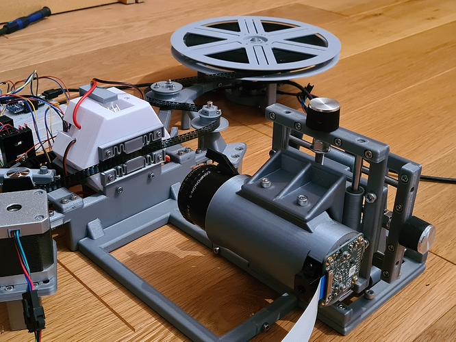
The lens that I am using is the humble Schneider Componon-S, 50 mm, which has been discussed before in this forum. Originally an enlarger lens, it delivers a very good image. Be aware that there is a light pipe build into this lens that you will need to cover up if you use the Componon-S as an imaging lens. One can buy these lenses used quite cheap, and it is still produced by Schneider, as far as I know. I bought mine in the 80s for my color lab I had at that time…
Here’s a picture of how I use this lens:
As you can see, the basic configuration is a 1:1 image path. That means that the distance between film gate and lens is about the same as the distance between lens and sensor chip, and both distances are approximately two times the original focal length of the lens. In fact, the focal length is 50mm, and the distance between the lens mount and the camera sensor is 91.5 mm. The Schneider Componon-S 50 mm has the best optical performance if you operate it at a f-stop of 4.0; lower values start to blur the image, while with higher f-stops than 4.0, the Airy disk gets too large.
The Schneider Componon-S 50 mm was designed for 35 mm film, so the distorsions for Super-8 are negliable. I do own also a Schneider Componon-S 80 mm, this was designed for the 6x6 cm format and might be a perfect lens for digitizing 35 mm with overscan. Anyway, I can really recommend these lenses.
Of course I do not only ‘import multiprocessing as mp’. I utilize at different places in the processing pipeline quite different schedulers to speed things up. For example, one of the simplest schedulers is the one utilized during resizing of the source images. Here, every image gets it’s own task and resizing the whole image stack is performed in parallel (my PC has 12 cores, and I work usually only with 5 images). Another scheduler is used in the aligment section of the pipeline. Here, the whole image stack is split into pairs of images which then are processed in parallel. Yet another one (used in calculating the feature maps the exposure fusion is based on) cuts the images in appropriate smaller tiles and processes these tiles in parallel.
Frankly, I am just fine with the speedups achieved. The pre-compiled original exposure fusion version right out of the opencv box needs on my hardware for my typical use case (image stack of 5 images with 2016 x 1512 px) on the average 1.105 sec, and my own version, running within the Python interpreter, needs 1.424 sec for the same task. That is only about 30% slower than the reference implementation and probably as fast as you can get within an interpreted environment. If I would need a further speed up, I would probably opt to implement the whole algorithm on the GPU - I have done such things before, but that’s why I know that it’s a lot of additional work. So I probably won’t go into that, at least not in the near future. ![]()
