… picking up this thread again. Remember, the topic is the color gamut of Kodachrome 25 film stock.
Initially, I was way too simple-minded when doing these computations. In fact, I actually started this thread in the hope to find more information on this diagram:
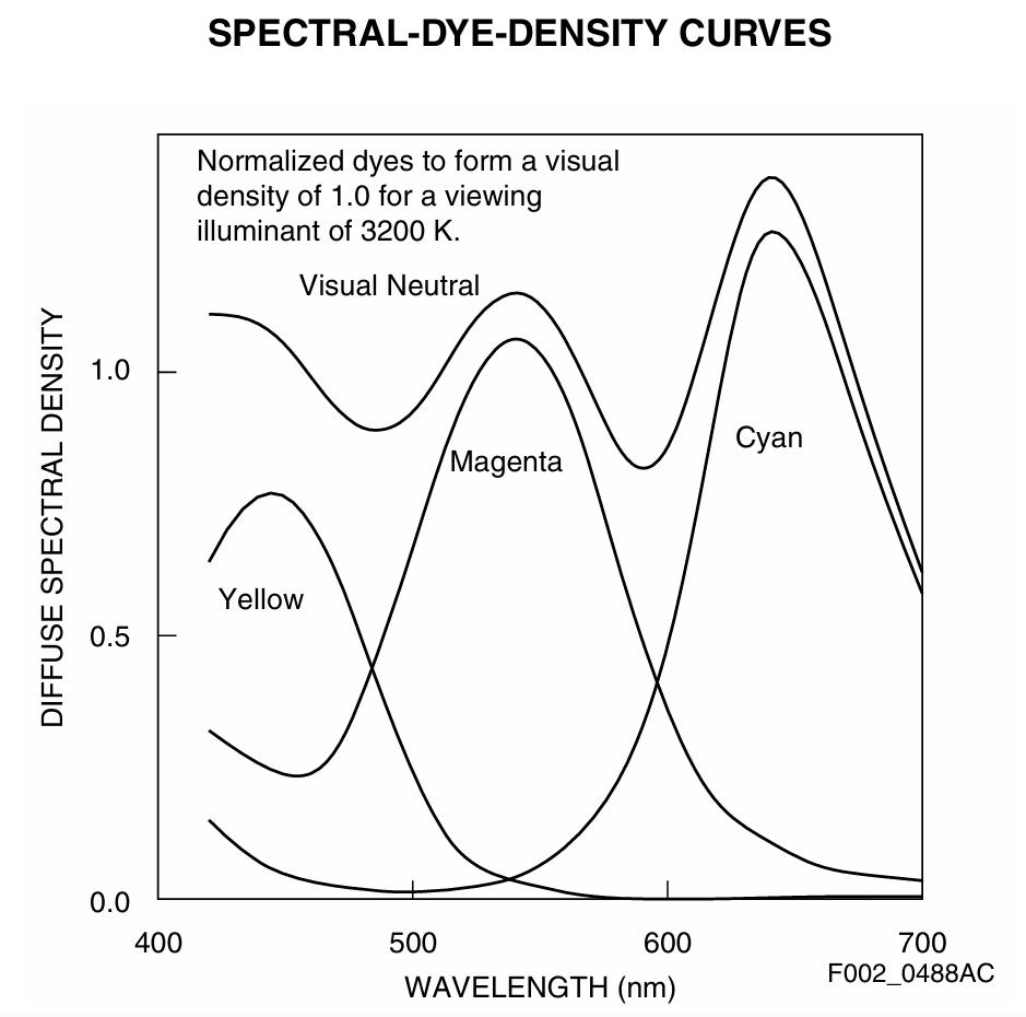
and how to interprete this data. I continued in parallel my journey through the internet to find out more about these data sheets - that turned up practially nothing until today.
So… - I came up with my own interpretation of the Kodak datasheets. And, as the characteristics obtained do not look too weird, I want to report here at what I arrived until now.
First, I decided to ignore the “for a viewing illuminant of 3200 K” comment on the graph. The “Visual Neutral” curve of the graph is a close approximation of the spectrum one would obtain with a grey card and with illuminant E. Which would be just a constant horizontal line. The “Visual Neutral” is a little bit wavy, but resonably horizontal oriented.
Next is the observation that the y-axis is called “Diffuse Spectral Density” - so these might not be absorption spectra at all. Assuming instead that these are really densities, one would have
absorption = 10**( -density(lambda) )
as a formula for the absorption of a single layer of film. Of course, we have three of them.
The next question to answer is the variation range of the dye densities. Well, this data is not given in the Kodachrome 25 data sheet. I made the following shortcut: there is a density diagram in the data sheet, but only for RGB data:
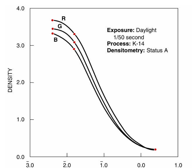
I digitized the curves at the red dot positions and obtained:
D_min   = 0.193

D_max_R = 3.676
D_max_G = 3.446
D_max_B = 3.319

D_max_R_lin = 2.900
D_max_G_lin = 3.082
D_max_B_lin = 3.304
Here, D_min is the density of the film base (the rightmost dot in the diagram), and the D_max values are the maximal densities possible (the three leftmost dots). The D_max..._lin value are the three dots at the end of the linear part of the curves.
Tactically, I opted as density range for the dyes, [D_min:D_max], with D_max given by
D_max = (D_max_R_lin+D_max_G_lin+D_max_B_lin)/3 = 3.095
With the above absorption formula, this gives me for the whole range of densities a transmission value for each wavelenght. For example, the yellow dye yields the following transmission graph:
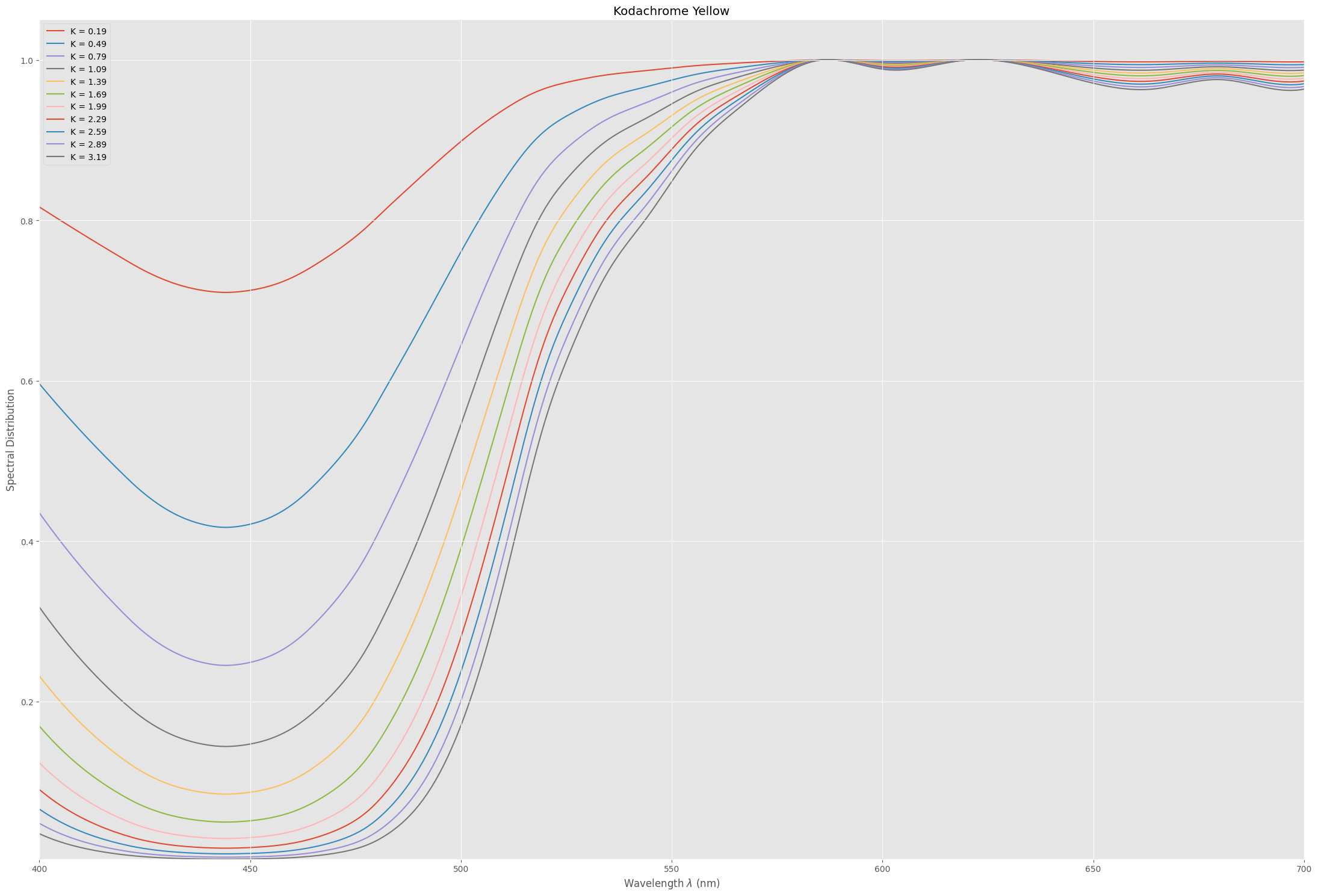
Note that here the difference between the yellow and blue part of the spectrum is getting stronger for larger densities (darker colors). So already here we see a characteristic of the subtractive nature of classical film: darker colors appear more saturated. That looks promising…
Next, let us look at the whitepoint of Kodachrome. That is, the “Visual Neutral” curve from above. When viewed with a normal projection lamp (around 3200 K), “white” will be somewhat yellowish. However, the visual system of the observer will take care about this, via a color adaption transform. I opted not to use a projection lamp for the simulation, but again my Osram SSL LED as illumination source. The differences are neglegible. Let’s have a look on how the “Visual Neutral” with varying densities behaves. For this, we are utilzing a classical CIE-diagram, operating in sRGB for display purposes:
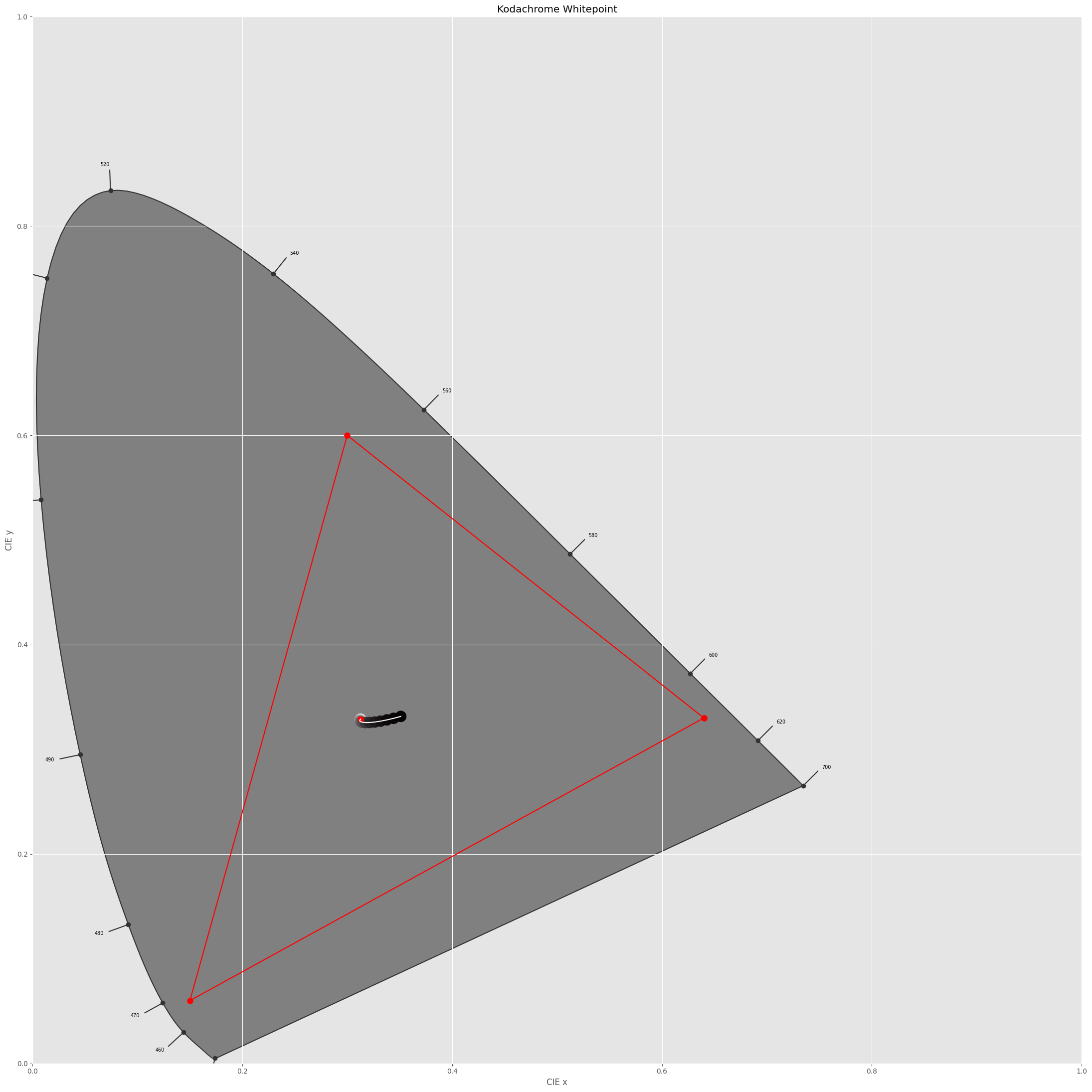
A short regression is in order here: this diagram displays the chromaticity of all colors a human observer is able to perceive. The red triangle marks the boundary of colors which can be displayed correctly on the chosen color space, in this case sRGB. Colors outside the red triangle are only approximations of the real color. The red center dot marks the whitepoint of the color space.
Now, there are basically no colors displayed here. That is actually to be expected, as we are mapping "Visual Neutral"s, that is “whites”, into this diagram. Let’s zoom into the center part of this diagram:
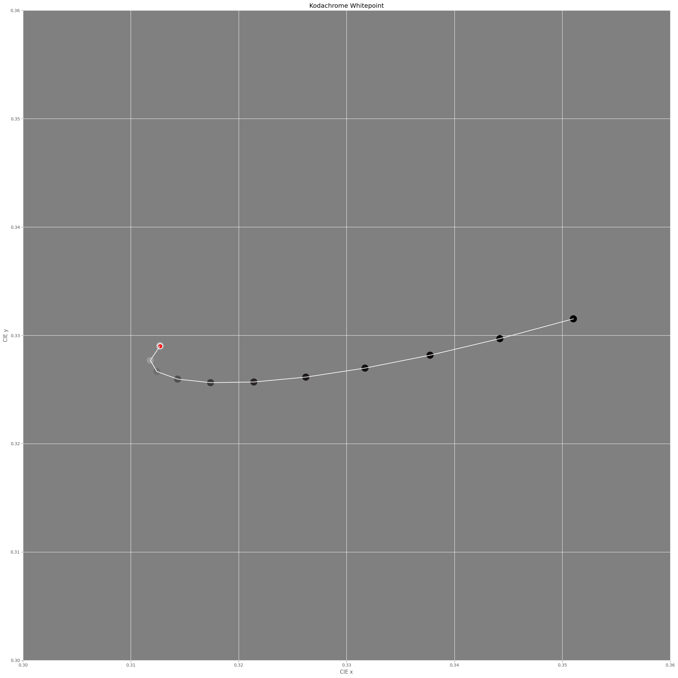
The red dot marks the whitepoint of our display color space, and as we can see, a lot of the brighter data points land directly where they should land. But, looking toward darker intensities, we observe a drift (mainly towards the yellow) of the Kodachrome whitepoint. Since shadows usually have a tendency to be more blueish anyway, that is actually probably not too bad.
Let’s check how our film dye layers (Magenta, Cyan and Yellow) perform. Varying the density of the dye layers from [0:D_max], where D_max is given by 3.095, we obtain the following diagram:
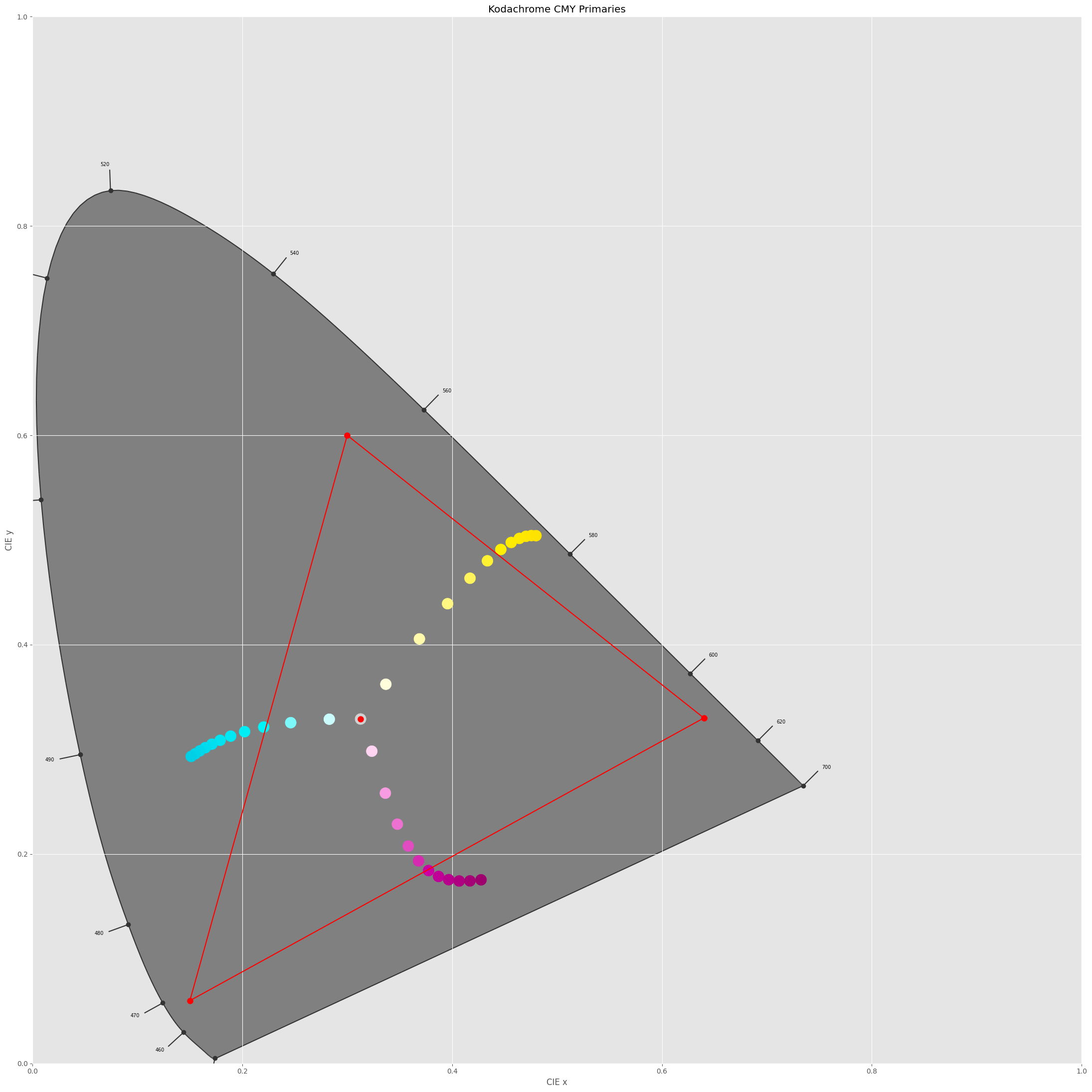
Remember, the colors outside the red triangle are only approximations to the real colors, as they are outside of our display color space. Clearly, the dye colors go outside this range for higher dye densities. Note that the primaries do not move on straight lines, as it would be the case for an additive device (your computer screen, basically, or your digital camera).
Ok, onto the red, green and blue colors. The computations yield the following:
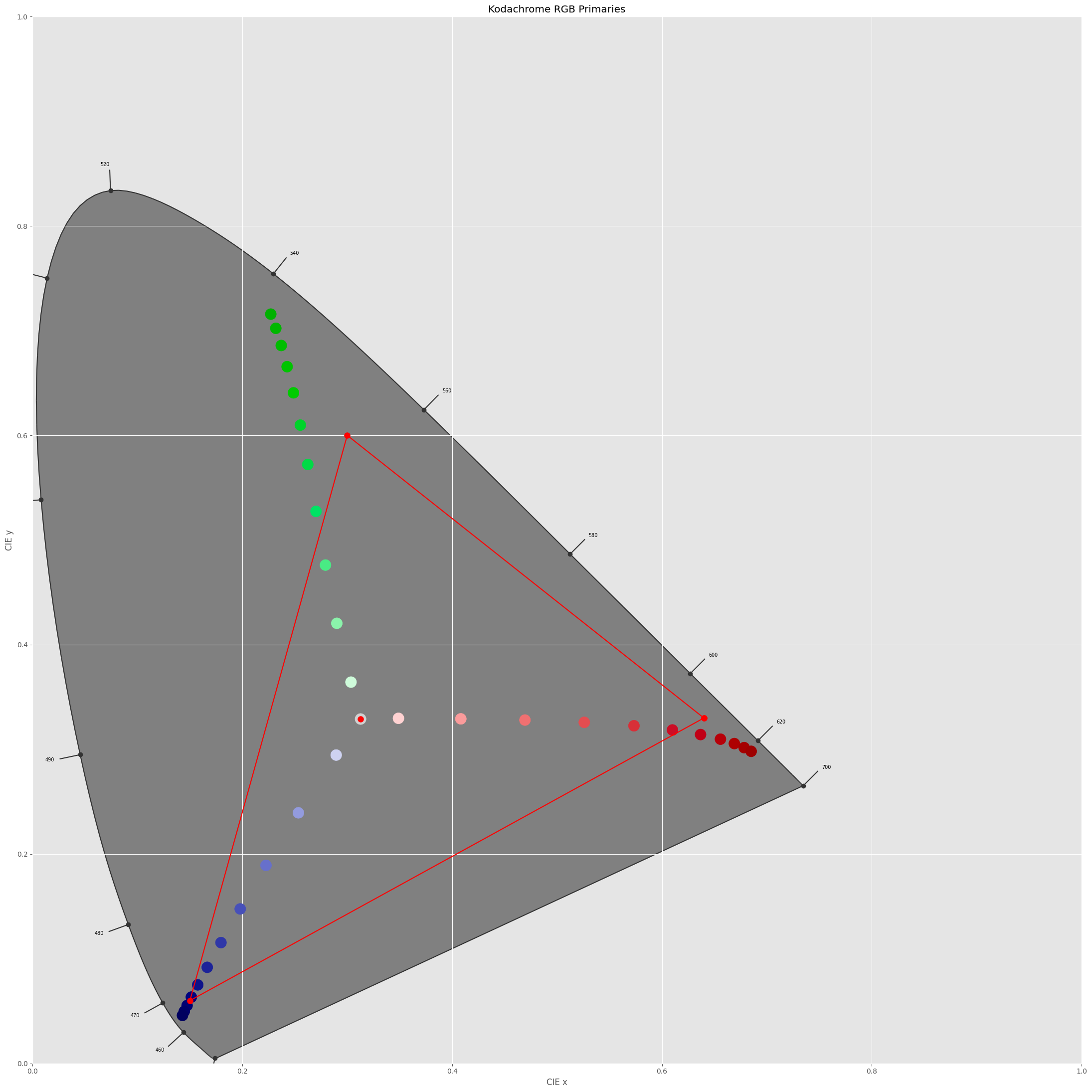
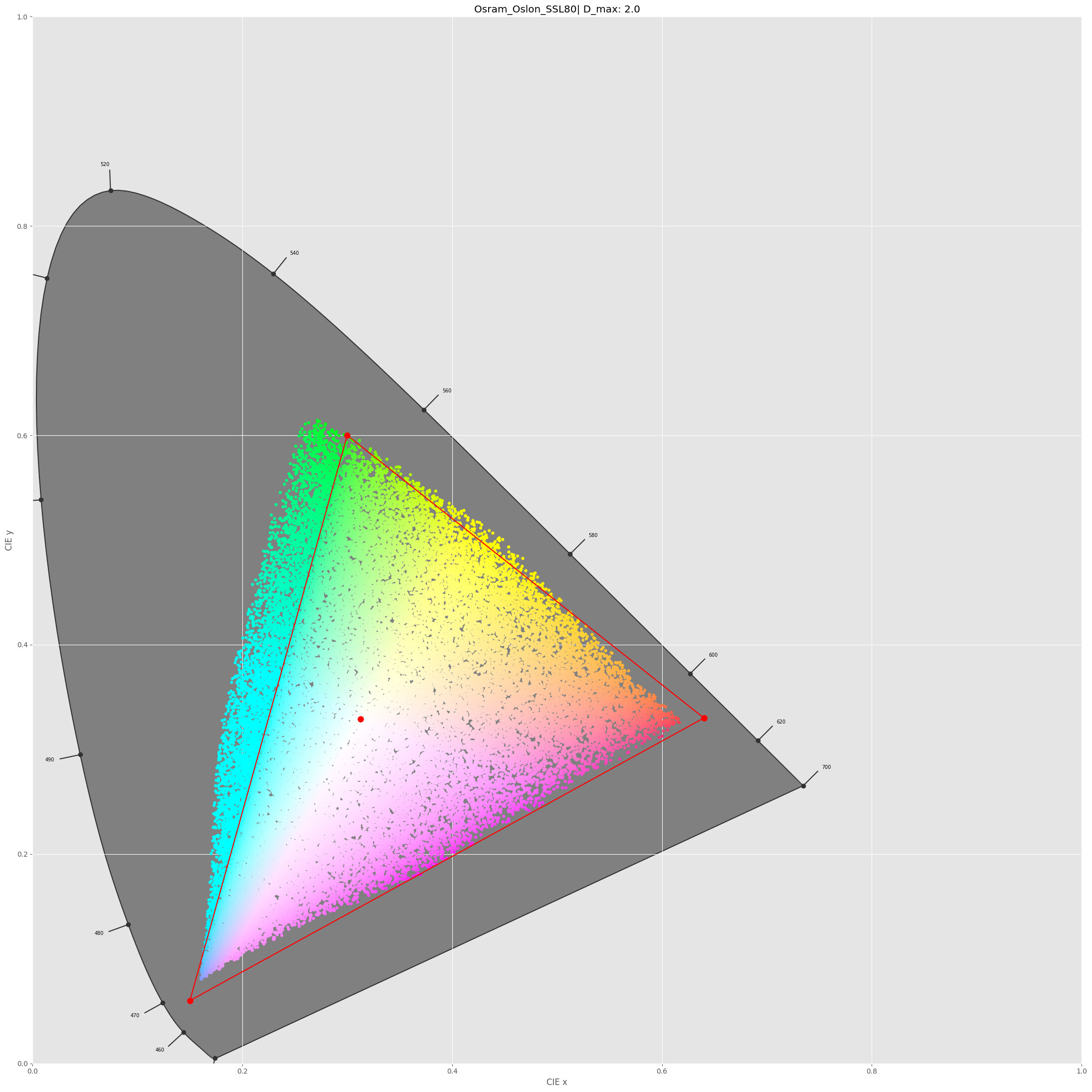
Especially in the green part of the color space, the Kodachrome colors end up way outside the sRGB color gamut. To get a better impression of the size of the Kodachrome 25 color gamut, I created
50.000 random colors and mapped them all into the CIE-diagram. This is what I obtained: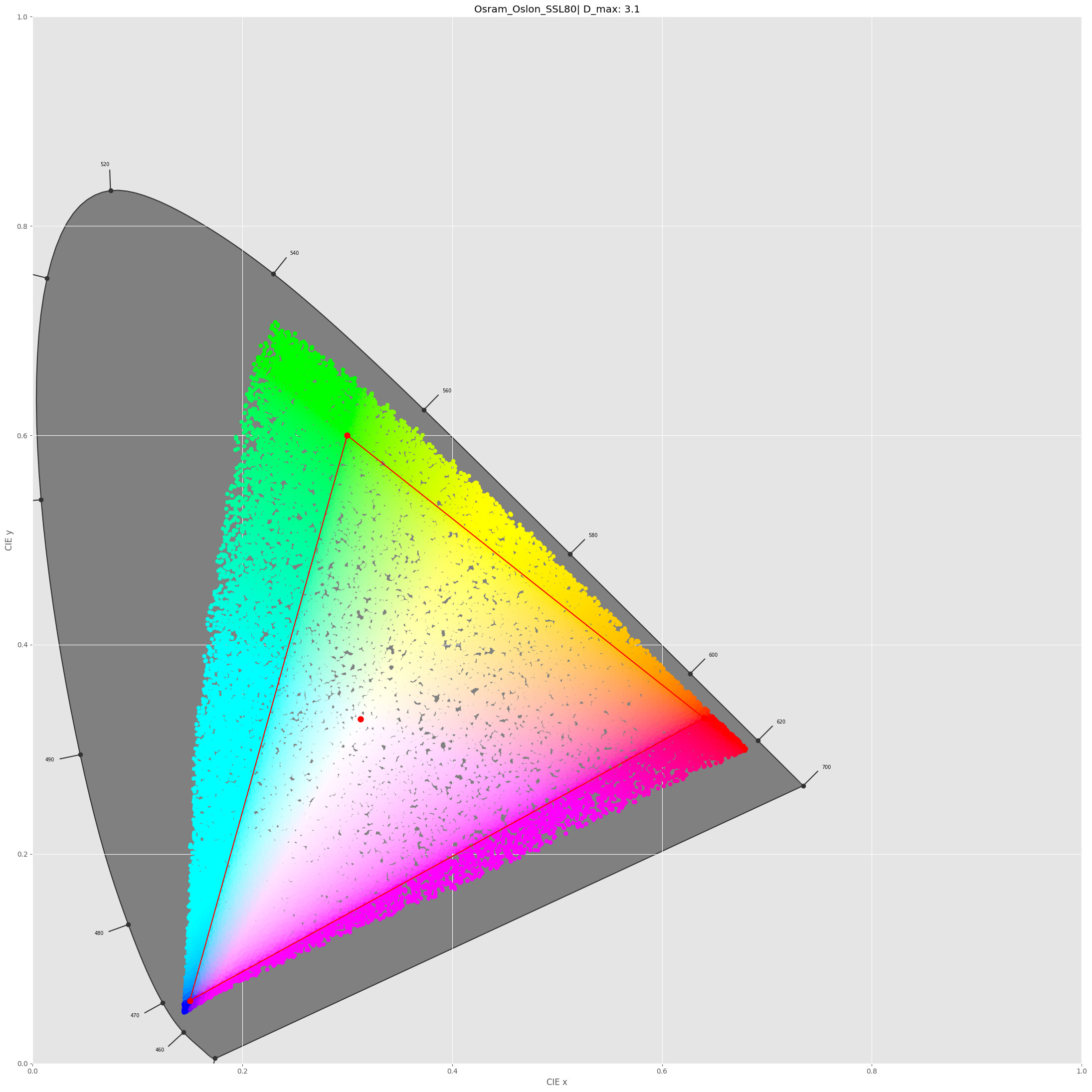
That in fact looks more correct than my initial simulation based on a wrong approach. And quite similar to the only Kodak CIE-diagram I could find (the right plot below):
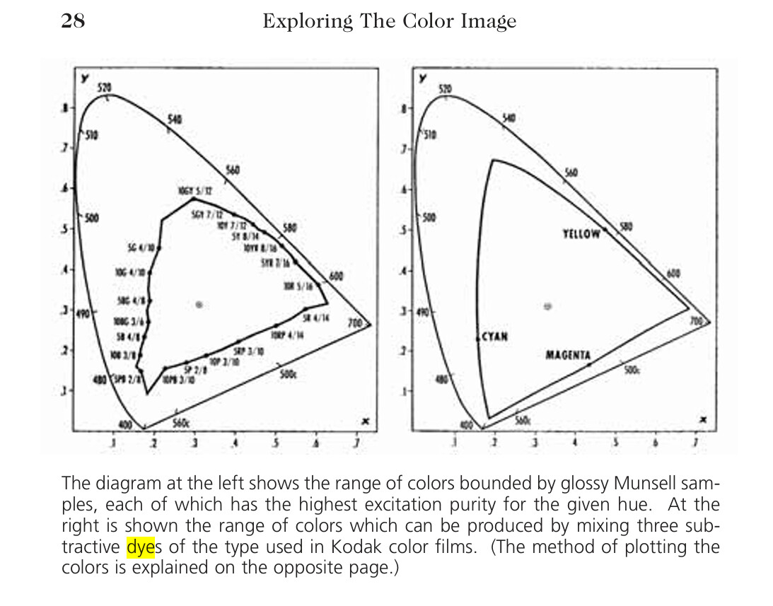
(This is from an old Kodak-publication, “Exploring the Color Image”.)
So: the color space of Kodachrome 25 film stock is greater than the sRGB display space. At least if my interpretation of Kodak’s data sheet and my simulations are reasonably correct.
One final note: the size of the color space depends mainly on the density range. I used a rather large range in the above simulations. If I constrain the density range sampled for the test to only [D_min = 0.5: D_max = 2.5] (positioning the test colors more on the linear part of the density curves), the color space shrinks a tiny bit:
That’s if for now. The whole exercise above should allow me to create a virtual Kodachrome 25 color checker chart - which in turn should allow me to compare scanning quality with whitelight LEDs vs discrete narrowband LEDs - that’s the next step here. Again, the above simulations are based on a lot of guesswork - so any comment is highly appreciated.