New HQ Raspberry Pi Camera with C/CS-Mount

jankaiser · May 5, 2020, 4:55pm

It’s great to hear about some actual first hand experience with the new camera!

The 16mm lens you were using isn’t by any chance the 16mm lens that is offered alongside the HQ camera? I would love to hear if anyone has had a chance to try that or the 6mm lens (with respect to 8mm film in particular).
I am still looking into what lens to get for my 8mm film scanning setup (somewhat on a budget), so I was reading up on the 6mm and the 16mm lens. In The Official Raspberry Pi Camera Guide they recommend the 6mm lens for macro photography, which seemed odd to me. From what I gather from these data sheets (6mm data sheet / 16mm data sheet) their MODs are the same at 0.2m. That should make the 16mm more suitable. Do please tell me if I am mistaken.

WDaland · May 5, 2020, 5:13pm

Would this help?

cpixip · May 5, 2020, 5:35pm

@jankaiser: well, yes. I was using the “offical” 16mm lens. The image of the camera box I posted above is actually the shortest distance you can focus this lens (with the lens screwed in fully).

The lens is not that bad, but if you look closely on the color chart also posted above, you can see some barrel distorsions.

In case you want to image the Super-8 frame with this camera chip and lens, you will need somehow to extend the distance between lens and chip.

For the v1- and v2-cameras, the sensor size is actually just about the same size as the frame area (plus sprocket) of a Super-8 frame. Therefore, any lens can be used in an arrangement which images the frame 1:1 onto the sensor chip. Simplifying a little bit: given a lens with a focal length f, you get this 1:1 imaging if the distance between sensor and lens is 2 time f. And you will discover that the distance you need between lens and Super-8 frame is also 2 times the focal length of your lens.

Now, there’s a twist hidden here. Lenses are manufactured to work optimal in a certain regime. So, of course you can use a normal lens for macro photography, by using just extension tubes. But you won’t get the optimal lens performance out of this setup. Your normal lens is optimized for a distance of one focal length between lens and camera chip. That is the reason some people reverse the lens they are using in doing macro photography.

The choice I made was to pair the camera sensor with a Schneider Componon-S 50 mm. For two reasons: first, this is an old enlarger lens which is optimized exactly for the distances I am using it. Second, I have two of these lenses available from my old analog photolab

Whether the Raspberry Pi foundation lenses perform sufficiently well in macro conditions needs to be seen. If I would have to choose between the 6 mm and the 16 mm version, I would probably go with the 16 mm version. First, it is easier for the optical designer to optimize a long focal length, so I would expect the tele-version to have less a distorsion problem than the wide-angle version. Second, if your camera would be in the 1:1 setup (which is not the appropriate one for the new HD-camera, because the sensor size is larger)it would be about 32 mm away from the film gate with the tele-lens, but only 12 mm away when using the 6 mm wide-angle lens. More space around the film gate is usually of advantage, because, for example, you might want to clean it occationally.

All in all, I would recommend not using these kind of lenses, as they are designed to be used in surveilance applications - you will probably have a better image definition if you use a better lens. Even the above mentioned Schneider Componon-S 50 mm has a sweet spot: you get the sharpest image definition at an f-stop of about 5.6 to 8.0. Lower f-stops start to blur the image, quite noticable already at 2k to 3k scan resolution, because the outer parts of the lens focus on a different plane that the central parts. Pushing to higher f-stops leads also to defocusing because the light rays are bend around the small f-stops. All in all, one probably just has to try out the lens.

cpixip · May 5, 2020, 6:01pm

@WDaland: wow, that’s an interesting find! Waited for something like this to happen for years. That might give the opportunity to optimize the available Raspberry Pi cameras for the task at hand, namely scanning movie frames with optimal fidelity. The v1- and v2-sensors are already supported, but frankly, they only can be used with their original lens. The new HD-sensor is a different beast and will be supported shortly. Cool

jankaiser · May 6, 2020, 10:50am

@cpixip: Thank you so much for this great insight! It’s very helpful.

I’ve seen the Schneider Componon-S 50mm being a fan favourite around the Kinograph forum for a while now. I had always assumed it’s on the pricier side, but it seems a decent used one can be had on eBay (in Germany) for as little as 50€. This puts it in the same ballpark as the 16mm Raspberry Pi lens and presumably makes it the better “deal”.

Have you had the chance to try the Componon on the HQ Camera as well?
I’m guessing it would need at least a 43mm filter thread to C-Mount reverse adapter to mount the lens in good setup for 8mm film scanning.

cpixip · May 6, 2020, 5:13pm

Well, have a look at my current setup, utilizing a see3CAM CU135 ( AR1335, sensor size about 1/3.2", or 4.54 x 3.42 mm, diagonal 5.68 mm, max 4096 x 3120 px), mounted onto a Novoflex bellow via a 3D-printed adapter. On the other side, the Componon-S 50 mm is placed - not in reverse mode.

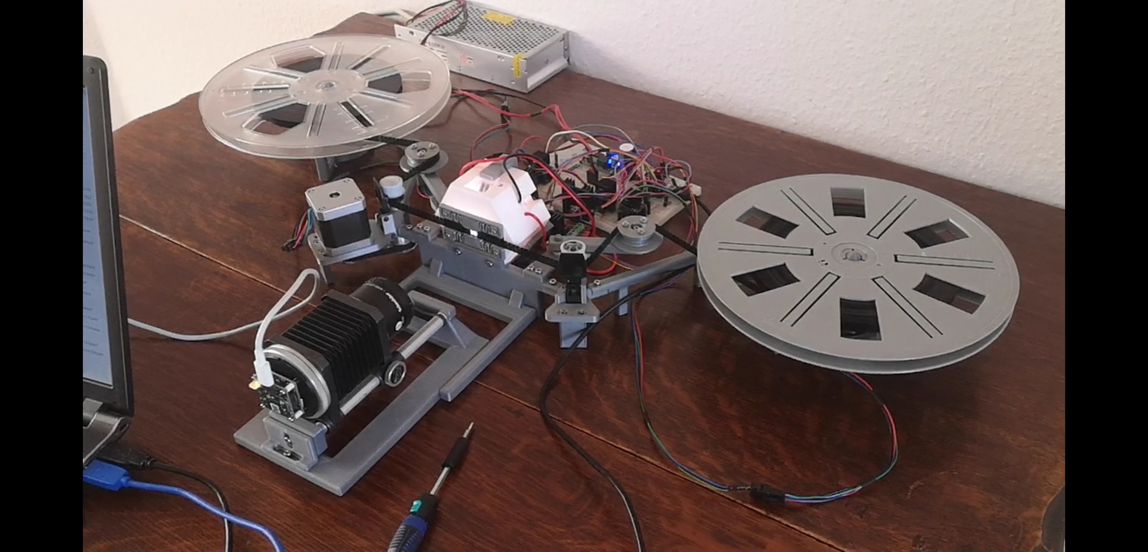
As you can see, the distance between sensor and lens is about double the size of the focal length of the lens, and the distance between lens and movie frame is about the same. Such an optical setup leads to a magnification scale of about 1:1. In truth, the optics are adjusted to a scale factor of 1:1.7. So the camera sensor sees an area of about 8 x 6 mm. This allows me to image the sprocket neighbouring the frame and have a little headroom for the frame position. The actual camera frame of a Super-8 movie is 5.69 x 4.22 mm, the projector is supposed to use only 5.4 x 4.01 mm of the camera frame.

Now, I have used the same setup with the Raspberry v1-camera (OV5647, 1/4", 3.6 x 2.7 mm, diagonal 4.5 mm, max 2592x1944 px) as well as the v2-camera (IMX219, same dims as OV5647, max 3280x2464 px). For these sensors, the lens only has to be moved a little bit to get the same scale as with the see3CAM.

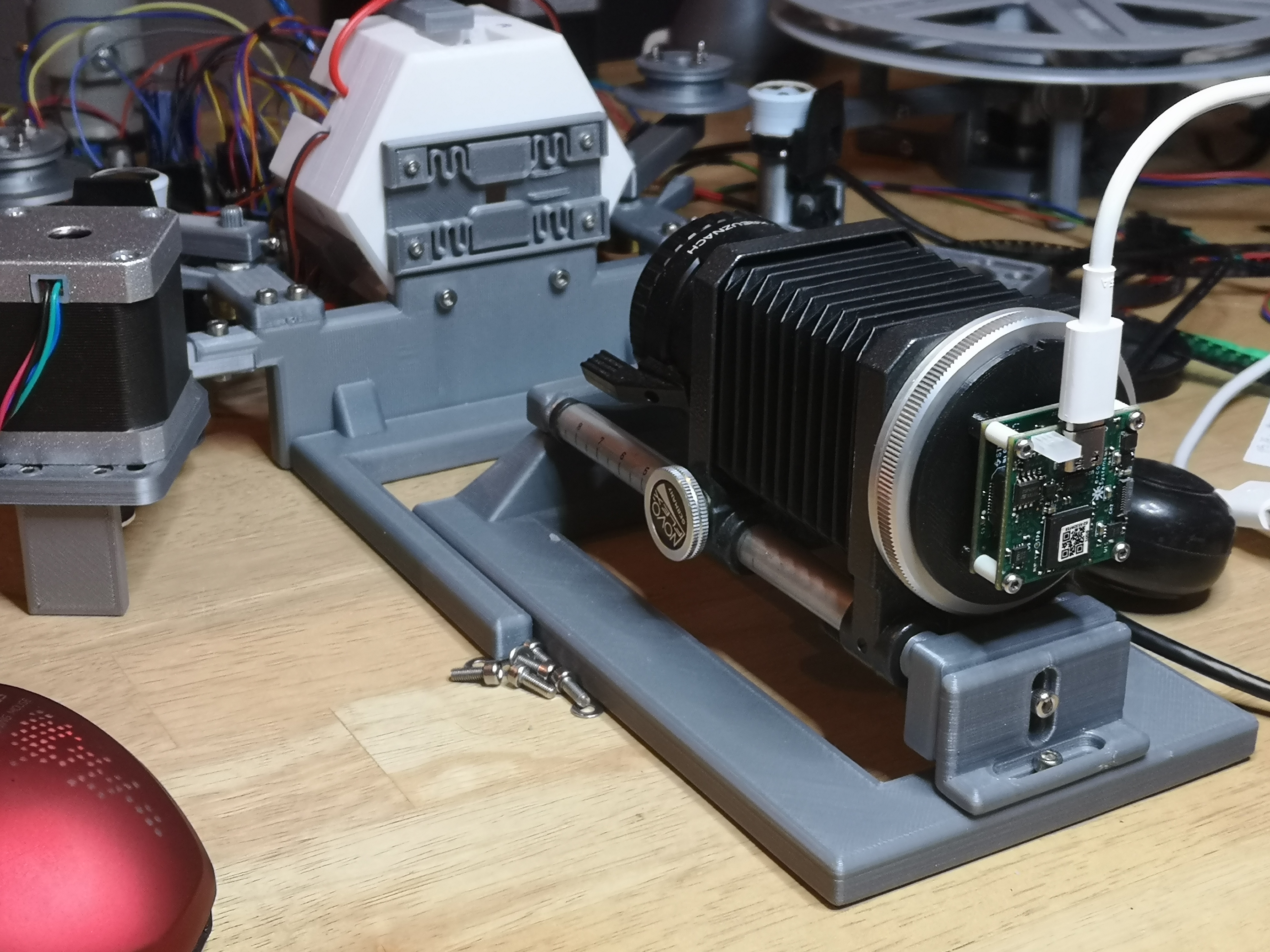
Here’s a more detailed view of the see3CAM mounted on the 3D-printed adapter which fits directly into the standard Novoflex mount:

I would prefer to use the same setup for testing the new Raspberry HD-camera (IMX477, 1/2.3", 6.17x4.56 mm, diagonal 7.66 mm, max 4096x3040 px), but the bulky C-mount of the camera is getting into the way of designing an adapter. Currently, the only option I see is to unscrew the whole aluminium mount and just use the bare sensor - I am not sure at the moment if I want to go along that path. Otherwise, I might opt to design a totally different camera setup.

Both routes will take some time, I am afraid, as I am currently using the scanner to digitize Super-8 material. I would also need to partially rewrite my old software to handle an appropriate camera mode for the new HD-camera. So it will take some time for me until I can share scan results with the new camera chip.

I am currently using the see3CAM in a resolution of 2880 x 2160 px, running at about 16.4 fps. From the specs of the Raspberry HD-camera, I think you would get maximal 10 fps out of the HD-camera at that resolution (in fact, I got about 7 fps with my python-based client-server software). So frame-rate wise, the new HD-camera is not better than my current setup.

My primary goal is to do fast HDR-scans - and the major bottleneck here is the time a camera needs to reliably settle onto a given exposure value. Not sure whether the new HD-camera behaves in this respect better than the old ones. Maybe the new libcamera-interface is helpful here. I will update on this as soon as I know more.

cpixip · June 21, 2020, 6:29am

ok, here’s the promised update on the Raspberry HQCam:

Raspberry Pi cameras feature different processing pipelines for still and video imagery. In fact, there is also a third pathway, namely output of raw sensor data, but it is prohibitively expensive in terms of scan speed and post-processing time.

The Raspberry Pi HQCam is based on a sensor mainly intended for video application, which is reflected in the available “camera modes” of this unit - only two of the four modes listed feature a still image pipeline, but all are available to output video.

The original sensor resolution is 4056 x 3040, but the maximal frame rate is only 10 fps at that resolution. The most reasonable mode to use is half of that resolution, 2028 x 1520, which is specified with a maximal 50 fps. This mode is also binned with 2x2, so it reduces the sensor noise by a factor of two.

The maximal frame rates specified are only achievable in video mode, because in still mode, the Raspberry Pi cameras need to capture actually several images before outputting a single result (mainly due to the automatic tuning algorithms adapting to the scene which is photographed).

This means that the data coming from the camera is MJPEG-encoded. So the data is heavily processed before it is available for use. However, people have seen characteristics in the raw data (mainly certain noise characteristics) which indicate some image tweaking is happening already at that sensor level - so chances are that even the offical “raw” image delivered by the sensor has already some (mainly noise-reducing) image processing applied.

However, the MJPEG encoding available with this sensor easily outperforms the encoding which is available with the v1- and v2-cameras of the Raspberry foundation. The encoding quality is reasonable already at a quality setting of 5%, and it increases drastically when the quality is raised above about 20%. Visually, there is no difference noticable with a quality setting of 60%, compared to a higher quality setting of, say, 95%.

The HQCam can be accessed with the usual software available, provided the OS is up-to-date. Access via raspistill and raspivid in a film scanning project is prohibitive slow or complicated (make your choice), but access via the picamera lib is fine - even so this library hasn’t seen any major update for quite some time.

The color separation of the new camera is fine, but the automatic whitebalance seems to be not as good as with the v1- or v2-cameras.

Optically, this is the first sensor from the Raspberry Pi foundation which is designed for attaching arbitrary lenses. The older v1- and v2-cameras feature a micro lens array designed for the working with the mobile phone lenses supplied with the camera. If you exchanged the lens of the older Raspberry Pi cameras with a lens with a different focal length, you ended up with color shifts and desaturation effects which are impossible to correct in post production. While the v1-camera performed here substantially better than the v2-camera, this issue is totally gone with the HQCam.

Mechanically, the camera features a machined block with standard connectors for lenses and tripods. Integrated into this block is also the IR-stop filter, so you can attach basically any lens you have available. I am using the trusted Schneider Componon-S for scanning purposes.

The outline of the new camera (angled, larger spatial footprint) makes it somewhat more complicated to design a housing or mounting for an existing design, but it is not too challenging.

For my specific application - HDR-scanning of Super-8 stock - it is mandatory that scanning and processing is reasonably fast. Standard Kodachrome film stock for example has a dramatic dynamic range, which is difficult if not impossible to capture with a single exposure. So several different exposures need to be taken of each single frame in order to capture the full dynamic range of the film image. This leads to huge amounts of data to be captured, transfered and processed. The most reasonable resolution to work with in the case of the HQCam is 2028 x 1520. In my setup, this gives me capture times of about 1.5 - 2 seconds per frame, with about additional 1 to 3 seconds for combining the different exposures via software (this time increases quadratically with image size).

Here’s an example of a HQCam capture:

It is a single frame from a Kodachrome movie, recorded in the 80s, which I got from ebay for testing purposes. The lower central image is the final output image, the surrounding images are the raw captures from the HQCam, spanning a range of 5 exposure values. Clearly, at least this huge range is needed to capture all the information available in the film frame.

The different exposures were not realized by switching the HQCam to different exposure values. It turned out that this takes way too long time. This is a behaviour which was already noted with the older Raspberry Pi cameras, but it seems that the new HQCam is even slower to respond to changes in exposure time. So instead changing the exposure time of the camera, the LED-light source was switched rapidly to different light settings for capturing the different exposures. The HQCam was run at a constant exposure time of 1/32 sec.

peaceman · June 21, 2020, 6:27pm

Thanks for the excellent info. I am still working on my rig and have limited time for hobby projects right now, but I was impressed by the dynamic range I found in the HQ Cam’s raw stills. However, 23 MB per image is a lot, and the DNG processing takes time and effort.

I captured a bit of raw video too, but failed to find anything that can decode it. The raw video should still have 10 bpc (and stills 12) — but how to convert it into something readable?

cpixip · June 21, 2020, 9:11pm

Well, I guess that depends. I am nearly always working with the picamera-library, and here, if you switch the camera to raw mode, you simply get the raw-data, together with a preview jpg, as a sequence of images out of the PiCamera-module. All you need to do is convert the raw Bayer image into something which resembles a more usual RGB-image.

Well, for this conversion, I wrote my own raw-converters in Python for the v1- and v2-cameras (each camera needs its own decoder), as I needed at that time the raw camera image in order to do lens-shading corrections and other stuff. I did not bother to write a new one for the HQCam, as I had no demand yet for one. I have not seen any Python code which does this in the wild either.

Besides the picamera lib, the other option to get raw image data out of the HQCam is to use “raspiraw”. This software seems to be recently modified to work with the HQCam, and it tries to write 12MPix, 12bit image data unpacked into 16bpp raw files. These files can be converted from the raw Bayer pattern they contain to something more usable via the “dcraw” program.

As far as I understand it raspiraw can be run also in a “video mode”. Never done this personally, but I guess in this mode raspiraw simply packs the raw frames one after the other into a large file. So you might try to cut out a single frame (each frame is of fixed size, so that’s not too difficult) and decode it after this with dcraw. But again, just guessing here, never bothered working with raw video or the Raspberry Pi Foundation software bundle.

A guy which is very active on the Raspberry Pi Camera Forum is Hermann Stamm-Wilbrandt. His scripts and insights might be of further help here.

peaceman · June 22, 2020, 7:46am

Thanks so much for these leads and hints.
GitHub - schoolpost/PyDNG: Create Adobe DNG RAW files using Python. Works with any Bayer RAW Data including native support for Raspberry Pi cameras. is what I used for IMX477 Debayering and it worked very well for stills).

For catpturing raw video, I had only tried raspivid with the -r option quickly.

Anyway, first step now is to get familiar with the picamera-library and python in general — haven’t ever touched python yet only C so far.

peaceman · June 22, 2020, 8:49am

Regarding JPG vs Raw quality, here are my first quick tests. This is a JPG “out of cam”:

And this is a JPG developed from the DNG I opbtained from pyDNG conversion:

And here is some detail comparison at 100%:

The reflexion of my desk lamp isn’t clipping in the Raw, and the detail of the bolt and nut are much better, too. There is also less fringing and the CA is correctible. Probbaly equally important, the lack of bilateral denoising in the Raw leaves a lot more detail, a temporal denoising approach should be much better here.

cpixip · June 22, 2020, 10:57am

To correct my quick comment a little bit:

Reading the description of raspiraw, it seems that the program writes out separate files, so no need to extract single frame from a larger file.

cpixip · June 22, 2020, 11:57am

@peaceman: very interesting results! Indeed, your comparision shows clearly the heavy image processing which is nowadays so common and so unavoidable with consumer sensors.

By the way - even the raw image of the HQCam has already some image processing applied. I have seen noise measurement of raw HQCam captures which hint to some spatial filtering applied at the sensor level. Also, for certain there are dead-pixel algorithms at work before the HQCam ships out it’s “raw” frame.

Usually, it is hard to get such information, as the chip manufacturer tend to keep their secrets, and nearly always impossible to switch them off.

Anyway - what would be very interesting to test (if you have the time and setup) is to see how the 12bpp of the raw image file compare against the dynamic range of a standard Kodachrome color-reversal frame with large shadow areas.

To elaborate: color-reversal film is usually exposed so that the lights don’t burn out. During projection, detail loss in the shadows is not so annoying than burning out the highlights of the scene. Also, our eyes as “consumer” of projected film frames are surpassing the possibilities of current sensor chips by a wide margin.

In order to reproduce highlight details in a scan faithfully, usually an exposure value for a single frame capture would be chosen so that the brightest image parts are still within the dynamic range of the full digital image path.

For example, I am working with 8bpp (and HDR later in my processing pipelinep). So my exposure is set in such a way that the sprocket hole of the film (which is pure white by definition) maps to something in the 240-250 value range (the maximum value representable with 8bpp is 255). With the 12bpp of a raw HQCam image, you probably could go up to values of 4000+ or so for pure white.

Now it would be interesting to see how good the performance of such an exposure setting is performing not in the highlights, but in the darker image areas of a frame. Specifically, how far can you go toward darkness?

There are two interesting points here - first, there will be more noise in the lower bit channels of a capture. This will raise the noise floor in dark, dense image areas, as compared to other areas. Another point to look at would be the limited amount of bit variation available in these dense film areas. Namely, only a few bits of the image data will change here. This could lead to banding and quantization artifacts (it might not - that would be an interesting result).

From my experience, a normal Super-8 frame basically never shows real dense areas, even in very dark shadows. Usually, the black mask around the frame is the densest part you normally encounter (and you would probably not care to scan these areas in high fidelity). However, in a fade you might encounter really dark areas in the frame itself.

Well, it would be interesting to see the limits of a raw capture here, given the challenges of this approach - you have to cope with large file sizes, low transfer rates and the need to “develop” the raw frame into something displayable on todays 8bpp frames… (given, this last point is about to change with HDR-displays )

peaceman · June 22, 2020, 1:34pm

I’ll definitely run some Kodachrome tests once I got my light source sorted… currently trying to coat a ping pong ball with Bariumsulfate from the inside to make a mini “Ulbricht” intergation sphere. Lots of moving parts as you can see

Your HDR results (like above) look really amazing, especially considering that you use output-referred 8bpc files. I’ve been remotely contributing to a HDR algorithm on my job and remember well that scene-referred input files (DNG from an iPhone in this case) helped a lot with proper tonemapping — so that one could darken e.g. the bride’s white dress without making the sun go gray. May I ask how you are compositing your output files? Is that a manual or an automatic process? And doesn’t taking 5 brackets + merging + tonemamapping take a substantial amount of time & processing, too?
[Edit: You answered this already earlier — I had to re-read the thread, sorry]

Regarding the “developing” of the Raw files into something eye-pleasing, I hope I’ll be able to create a camera profile for ACR, and if I can’t, I’ll try to bribe some colleagues to do so. (Disclaimer: I am a Product Manager for Adobe Lightroom, and ACR is built “next door”).

But we’ll see — first step now is the light source and getting going with some python scaffolding.

cpixip · June 22, 2020, 8:41pm

Well, the short answer is that it is an automatic process.

But here are some more details about my approach. Some background information first: my first image processing algorithms were coded in FORTRAN 77, I later switched for tens of years to “C” (and occationally C++/Java/Matlab/VHDL), but I finally ended up in doing most of my work in Python now. Shows my age, I guess…

Initially, I actually implemented a real HDR capture pipeline with the Raspberry Pi v1-camera as a basis. That is, appropriate gain curves were estimated and a real HDR with image radiances was created from different exposures of a single frame. However, my hope to find some appropriate, generic tone-mapping algorithm for the very different material I had at hand did not realize in any way.

Having spend also some time researching the human visual system, it occurred to me at the time Mertens with others published their exposure fusion approach that this approach has a lot in common with the way our human visual system views the world.

Here’s what I wrote in another thread about this:

HDR / Exposure Bracketing

…

From my experience, the exposure fusion algorithm (Mertens/Kautz/Van Reeth) is the best bet on combining different exposures of a single frame into something which is “viewable”.

Most importantly, it is basicallly a parameter-free approach (there are parameters, and for optimal results, you want to tweek them together with the specific camera you are using). Once you find a sweetspot, it does not matter much if you scan differently exposed scences or even different film stock - the results look ok. Great advantage in my view.

The original authors of the exposure fusion algorithm did not discuss too much how their approach actually works. Here’s my take on that: if you come from a photographic background you know that it was usual stuff in an analog photography lab to brighten and darken certain image parts which would come out too dark or did not show enough texture. You would select a main exposure time for the print and place your hand or appropriately cut-out paper pieces over certain image areas which would come out too dark otherwise. After that, you would do an additional exposure to further locally darken image areas which would otherwise be too bright in the final print.

In a way, exposure fusion automates this technique: they devised certain image operators looking for regions in each of the exposures of a scene which are

well-exposed

have a good color saturation

or a good local image contrast

Now, for combining these areas of interest, they choose a well-know image combination algorithm which is pyramid-based and was initially proposed by Burt/Adelson in 1983. That is more or less the basic idea behind exposure fusion, as far as I understand it.

In any case, the best part of all this is that you do not even have to bother to understand or implement this algorithm by yourself (well, I did that anyway… ) - it is implemented as " cv.createMergeMertens ()" in the opencv computer library. If you want to look at exposure fusion and all the other options (HDR-creation + tone-mapping) the opencv library has available: the following link shows you example code in C++, Java and Python (OpenCV HDR algorithms ) which you can use as a starting point for your own software.

The above mentioned opencv-implementation is quite fast and usable, but I opted to write my own version. It is a little bit slower and but offers more ways to modify and tweak the basic algorithm. I am still in the process of optimizing this, but I am fine with the current results - especially because the process is fully automatic. No manual adjustments needed!

Here is my current work flow, with approximate timings included:

Insert the film into the scanner, fix camera exposure to 1/32 sec, set the resolution to 2028 x 1520, set red and blue gain to a fixed value.
Check for all 5 exposure values that the sprocket area is pure white, set analog and digital gain in such a way that in the lowest exposure setting the bright sprocket area shows values about 10 units less than maximum brightness. This ensures that any bright image areas of the film frame are properly recorded.
Start scanning. Scanning consists of advancing the film one frame, waiting a fraction of a second for the film and mechanics to settle, and than taking 5 different exposures in short succesion by dimming the light source over a range of 5 exposure stops. This takes about 1.5 - 2 seconds for the 5 exposures.
The images are transfered from the HQCam to a Pi4 which acts as a server to my LAN. Depending on the speed of the LAN, transfer might take additional 2 - 5 secs per film frame.
The images are received by a client software which stores them to a disk. Currently, the client is also responsable to trigger the next frame capture, which introduces an additional delay. All in all, I usually calculate that for every second of Super 8 stock (with 18 fps) I need about 40 sec to a minute for scanning the material. So this approach is quite slow on the capture side.
Once the capture is done, the set of five images are combined into a single output frame. The exposure fusion algorithm which does that is usually run not on the source resolution of 2028 x 1520 px, but on a smaller 1200 x 900 px resolution. At that resolution, it takes on my PC between 800 - 1100 msec to process a single frame. At full resolution of 2028 x 1520, the computing time for a single frame increases to 1900 - 2100 msec/frame. The 1200x900 px images are stored as a 16bpp RGB image on disk, with an average size of about 5MB.
A final post processing program takes the 16bpp images and crops them 80% to get a final output image size of 960x720 px. At this stage, sprocket detection and alignment as well as color correction and grading is done. Also, a slight sharpening step is included here. This pipeline needs less than a second per frame (But I have not timed it really). The pipeline outputs the final frame as 8bpp RGB image with a size of 960 x 720 px.

Now, for me, 960x720 px is a resonable output format for my purposes (my old “Revue” camera combined with Agfa stock is far away from reaching even such a resolution… )

As the capturing and processing is slow, lowering the resolution at appropriate times in the pipeline gives me some gains in terms of processing speed. Actually, as capturing and post processing run unattended (a whole film is processed with the same settings), I usually do the processing overnight, just checking the results in the morning.

Anyway, I am still in the process of optimizing the whole thing. As this is the fourth or more version of my film scanner, I might end up with something totally different in a few months time…

Hope this wasn’t a too long response to read. Good luck with your light source, and it will be interesting to see what raw captures the HQCam can achieve!

peaceman · June 22, 2020, 10:07pm

This was definitely one of the most exciting reads for me here, yet. Thank you so much for all the detail. I’ll keep you posted about my results…

jankaiser · June 22, 2020, 10:43pm

Super interesting, definitely something to learn from that is very helpful!

Do I read this correctly, that using multiple exposures and the exposure fusion algorithm allows you to essentially set the exposure once (say on the first frame) and then leave it, giving “good enough” results even if later scenes are not exposed quite the same?
I have actually been bouncing around the question of what to do about exposure (automatic vs. manually setting it to a fixed one once) for a while now. Never quite got around to it yet, though, because I’m still figuring out some of the mechanics on my build.

cpixip · June 23, 2020, 5:19pm

Yes, that is basically the case - of course, within limits.Let me give four further examples to illustrate that. The captures below are from the same run as the example above, with all settings unchanged. Here’s the first, rather extrem example:

Again, the center image in the lower row is the output result of the processing pipeline, slightly color-corrected and cropped with respect to the input images. As one can see, the central region of the film frame is most faithfully recorded in the -5EV image which is the leftmost thumbnail on the lower row. The same region is totally burned out in the +0EV image which is the right one in the lower row.

Let’s focus a little bit more on this central region - here are areas near the columns which were grossly overexposed already during filming. There is no structure visible here, the Kodachrome film stock was pushed here to the limits by the autoexposure of the camera. There is however still color information (yellow color) available here. You can see this if you compare these overexposed areas with the sprocket area of the -5EV capture. Here, the full white of the light source shines through. If you use a color picker you will see that in the sprocket area, we have about 92% of maximal RGB values. That is actually the exposure reference point for the -5EV capture and all the other (-4EV tp +0EV) captures which are referenced to this one.

In any case, the minimal image information available in the central region of the frame (which is just some structureless yellow color) is detected by the exposure fusion and transfered to the output picture.

Turning now to the right side of the frame, you notice a really dark area. Here, image structure can be seen only in the -1EV (top-right) and +0EV (bottom-right) captures. However, the little structure which is there shows up in the output image as well, albeit with a rather low contrast. Given, you might get a slightly better result by manual tuning, but for me, the automatically calculated result is useable (and less work).

Remember that the wide contrast range of this image has to be packed by the algorithm into the limited 8bit range used by standard digital video formats, convincibly.

Another point which is important in this respect is how the algorithm performs when there is actually a low contrast image - will the algorithm in this case just produce an output image with an even a lower contrast?

Well, it is actually difficult to find a scene in my test movie which has a low contrast. Here’s the closest example I could find:

Because of the low contrast, the capture with -4EV (top-left) or -5EV (bottom-left) is actually a perfectly valid scan of this frame. You would need only one of these single captures to arrive (with appropriate chosen mapping) at a nice output image. Some of the other exposures are even worthless, for example the +0EV image (bottom-right) which is mostly burned out in the upper part and can in no way contribute to the output image in this image area.

Now, as this example shows, the output of the exposure fusion turns out to be fine again. There is no noticable contrast reduction here. This is an intrinsic property of this algorithm.

To complement the above, here’s another example, again with the same unchanged scanning/processing settings:

This example frame was taken indoors with not enough light available, so it is quite underexposed in the original source. Because of that, the -5EV image (bottom-right), which in normal exposed scenes carries the most of the image information, is way too dark and more or less useless. However, the +0EV scan (bottom-right) is fine. Because the exposure fusion selects the “most interesting” part of the exposure stack automatically, the output image is fine, again.

(One question I would have at that point if I would have read until here - what about fades to black in the film source? The answer is that they work fine. )

Well, the Super-8 home movies seldom feature a finely balanced exposure setting; usually, they were shot just with the available light, mostly direct sun light. So here, in closing, is a typical frame a Super-8 scanner will have to work with: dark shadows mixed with nearly burned out hightlights.

jankaiser · June 25, 2020, 3:15pm

Thank you for the great examples!

One question that comes to mind: What happens if the frame you expose for (say the first frame of a roll?) is not exposed correctly? Does this cause problems later down the roll? Or is this not an issue at all in practice?

cpixip · June 25, 2020, 4:37pm

It is no issue at all with the process described. The important thing is that the whole exposure sequence is set to the light source of the scanner itself. In setting it, I do not care about the frame content at all.

The exposure is set with a measurement of the sprocket area, where there is no film at all. Actually, it was measured once and I have never changed it between scans.

As through the sprocket hole the full intensity of the light source is shining through, even the clearest film stock will have a lower exposure value anywhere else in the frame.

This trick ensures that any structure in the highlights of the film source does not overwelm the capture device (at least in the -5EV exposure).

Now, any other structure present in the scanned film will be darker, actually much darker. Remember that color-reversal film is exposed to the highlights, not the shadows.

Capturing the shadow details is what the other exposures are for. You need to got into the darkness as much as possible.

The most challenging film stock I encountered so far is Kodachrome 40; here, the 5EV-exposure range is really needed for most of the film frames.

The darkest part of a scan is always the unexposed frame border, and if use a color-picker on one of the examples above, you will notice that unexposed frame border is slightly above the background in the brightest exposure (bottom-right).

In fact, my illumination can not go too much over the 5EV range, for various reasons. Ideally, I would like to push it a little bit further than currently possible. This has to do with the gain curves of the sensor.

Let me elaborate this a little bit.

I do not have any gain curves measured for the HQCam (yet), so let me use the gain curves of the Raspberry Pi v1-camera:

GainCurvesV1

The y-axis shows different EVs, the x-axis the range of 0x00 (0) to 0xFF (255) of 8bpp pixelvalues these EVs are mapped to. There is a more or less linear segment from 6EV to 8EV approximately. That is the “beauty range” of this camera.

Clearly, there is another range above 8EV, mapping to values 230 or higher, which is different from the main transfer range (from about 20-230). This is the range where the camera compresses the highlights.

Ideally, you would set the exposure in a scanner in such a way that the bright sprocket area (the light source itself) is mapped to 230 or less, not using the range where the highlights are compressed. If you just take a single exposure per frame, you actually can not afford this, especially because at the other, darker end of the range, shadows are compressed as well (in this example in the range of 6EV to 3EV).

The exposure fusion algorithm in fact ignores for each intermediate exposure the compressed regions in the highlights and in the shadows. The compressed highlight region is only used in the darkest exposure, and the compressed shadow region only in the brightest exposure.

I am setting the exposure reference in the darkest frame a little bit higher than 230; experiments have shown that this does not affect the visual quality of the scan at all and I gain a little bit more structure in the dark shadows this way. But I would love to have some slight additional head room here, say 0.5 EV or so. Can’t realize that with my light source, as the DACs have only 12 bit resolution and the LED color changes at different illumination levels pose an additional challenge as well.

I hope the above was not too technical. To summarize: the exposure in my scanner is never set/changed with respect to the film source. It is only set once, with respect to the light source. It is normally not changed from film to film.