Super-8 enhancement, progress report

Well, this is an interesting remark and certainly a possibility. However, the JPEG artefacts are very minor with the HQ camera operating at quality setting of 95. I checked that.

For speed reasons, I can not really switch to another image format as the only other, “better” format would be the full raw format. In fact, I tried this and compared scans with raw images to the image quality of the JPEGs coming out of the video port of the HQ cam. Not too much difference at my settings. But maybe my raw processing was not really up to the task…

The motion estimation algorithms are actutally working on the exposure fusion results. After exposure fusion, no JPEG artifacts are any longer present in the data, they are averaged over during the exposure fusion.However, the noise from film grain is still there. I am afraid that this is the main cause of the problem. So I am currently looking into better ways to prefilter selectively the source files before motion estimation to improve things. But progress is slow.

Indeed. Neither the exposure time (1/32), nor digital (1.0) or analog gain (1.2) are ever touched during scanning. Also, the color balance is kept at fixed values red = blue = 1.67 (this is an unusual color balance for the Raspberry Pi HQ camera, because I replaced the stock IR-filter with another one. Long story.)

1 Like

@cpixip but @PM490 consider this if you come from a DSLR
but consider this if you come from a DSLR
We all agree that when capturing, a shutter speed change is not immediately reflected and that you have to ignore a few frames before you get the one with the desired exposure value. This is due to the fact that the Pi camera is not a DSLR but rather a video camera that once initialized continuously sends images to the ISP. When an application “captures” an image it gets the current image at the output of this pipeline. Even if the processing is reduced to the minimum without auto functions (awb, shutter,…) you have to wait 3 frames to see the change of exposure. It takes longer of course if there is a feedback and some processing in the pipeline, for example it takes at least 8 frames to calculate an automatic exposure. So I think there is no reason why it should be different when you change your lighting, you say you wait 0.25s at 10fps, we are not far from 3 frames.

For HDR 3 or 5 in practice I do not notice any difference. The dynamic range of the HQ camera is not bad (it was quite different with the V1), HDR is mainly used to avoid burnt whites, just make sure that the dark image is largely underexposed, I go to -4EV.

For the focus it’s really very sensitive, I use a micrometer sliding table and I calculate a numerical
value of the focus quality. The adjustment must be accurate to within 0.1mm.

Finally for the dancing grain it is possible to send me the image sequence that I see if there is a difference with my avisynth scripts ?

@dgalland - you have a sharp eye! Actually, while rereading our discussion, I noticed that at one point in time I switched from the original maxial mode 3 resolution of 2028 x 1520 px to a slightly lower resolution of 2016 x 1512 px.

I cannot remember why and when I introduced this change. Here’s an enlarged view of a scan near the sprocket hole with resolution 2016 x 1512 px:

and here, for comparision, the same spot scanned with the original 2028 x 1520 resolution:

Well, I think the difference in sharpness is quite visible. Seems that the Raspberry Pi image stack does always a zooming operation, even when a simple cut-out operation would be sufficient.

Again, well spotted!

… while enjoying the pleasure of blown-up enlargements out of tiny Super-8 frames, here’s another example of the still image performance of my approach (capturing 5 different exposures spaced 1 EV apart, exposure fusing into an intermediate 16 bit frames, degraining the footage and sharpening):

This here

is one of the original exposures (the “prime scan”). There is the additional highlight scan

and this is the brightest (Stage 02) of the three different shadow scans:

The exposure fused image (normalized and gamma-corrected, otherwise it looks rather dull) looks like this:

Note how the image definition in the dark tunnel is improved. Also, the highlights are less blown out in comparision to the prime scan.

Degraining and sharpening this footage gives the following result (again, normalized and gamma-corrected):

The sharpening might be a little bit overdone (note the pronounced edge between dark tunnel and the bright dress of the child) but I like the improved definition on the faces of the people as well as the better visibility of the cracks between the stones. Actually, in those high-contrast areas, the “pixel dancing” is not noticable at all - this is only a problem in low-contrast areas where the film grain outpowers the image structure.

I don’t understand why you call the darker scans “higlight” and vice versa! For me three images would have been enough to ensure the result and the darker image could have been even darker.

Concerning the resolution and modes, yes, it is necessary to limit as much as possible the resize, that’s why I scan directly in mode 1 1500x1080, the only resize will be the one that will take place during stabilization.
I think you are making a confusion, mode 3 is the full non-binned mode with a maximum resolution of 4056x3040, it’s the mode 2 binned which has a maximum resolution of 2028x1520. Do you use mode 3 or mode 2 ?
The mode determines the resolution that comes from the sensor, then changing this resolution or defining a ROI causes a resize (not a crop)
So if you use mode 3 with a resolution of 2028x1520 there is a resize. I don’t know if the result is better than the mode 2 binned 2028*1520, you should make the comparison.
If you don’t specify the mode (mode=0) it is chosen automatically depending on the resolution and framerate.
I also noticed a curious thing when you have chosen the mode there is a maximum framerate that you can get in the application (see my table above with the experimental values). It is important to ask for this value, for example 19fps and you will get 19fps but if you ask for more, 25 fps for example, you will get less than 19!

Sharpening is a tricky problem, with avisynth there is a videofred recipe that gives an excellent result, something like this:
sharpened=source.unsharpmask(30,3,0).blur(0.8).unsharpmask(50,2,0).blur(0.8)
try it !

… some further feedback…

Well, I certainly agree that you need to wait at least 3 images until the exposure value has stabilized. However, I noticed with various different sensors a drift requiring much longer waits until the exposure had stabilized. Actually, this temporal behavior was different depending on what the combination of initial exposure vs. the target exposure was during testing.

These experiments were done long ago, but during that experiments I of course made sure every auto function of the image processing pipeline was switched off. Well, the processing pipelines might have changed in the intermediate time, I do not know the current status. Maybe the cameras react today faster than 2-3 years ago with exposure changes.

Let me remark that when you are using exposure fusion, you do not really need to get precise exposure times. As long as the exposures are consistent from frame to frame, you will not notice anything. The exposure fusion algorithm does actually not care what the real exposures are. This is different when you switch to real HDR work - here exact exposure values are normally required (You can estimate the exposure values after the fact, but that is noticeably more complicated). In case you want to upgrade later to a full HDR workflow, exact exposure values make your life easier.

In any case, the delayed and non-reproducable response when switching exposure times was the reason I abandoned this approach in favor for a tunable LED source.

Also, at least in theory, with a tunable LED source, you do not need to wait 3 frames, as there is no change in the camera parameters at all. The wait times in my approach are connected to the fact that I have not yet synchronized camera and LED source (this will have to wait for the next major update of the scanner).

Initial experiments with 8 bit DACs revealed that the dynamic range would be too low for capturing most Super-8 color reversal material, so I swapped the DACs out for 12 bit ones. Even so, the dynamic range is barely enough; especially towards the lower illumination levels, a single step in digital brightness results in a large difference of illumination. The five different exposure levels spaced 1 EV apart are the maximum I can currently realize with my 12 bit DACs and the LEDs chosen. Limits come from the available LED output (not enough power) and the color changes introduced by varying the current through the LEDs (this is a tricky one: basically, it is connected to the operating temperature of the LED in question. And of course, that temperature changes constantly at a rapid pace during scanning…). Lastly, even a 12 bit DAC is not really precise enough to cover a larger dynamic range than about 5 EVs.

Let’s step back a little bit. In fact, a lot of people do not bother to work with multiple exposures of a single frame, just use a single, well-chosen exposure. In this case, in very dark image areas you notice a reduced contrast with increased noise, and very bright image areas of the frame might easily burn out.

The reason for this can be understood with the help of the diagram below. It shows the response curve of a camera sensor - what pixel value (y-axis) it will output when exposed to a certain brightness (x-axis).

This is a typical camera curve - from cheap webcams to high-end DLSRs (not talking about the raw format here!) you will find a response curve very similar to this one.

Now, there are two parts of this curve where the response curve becomes rather flat; I am talking about the flattened parts of the curve in dark areas (-5 EV to -2 EV) as well as in the bright areas (anything above about 1 EV in the diagram). In these these exposure areas, a rather large difference in exposure will result in only a minor change in bit-values of the output image. Add the sensor noise into this equation and you end up in the dark parts of the image with noisy, rather structureless blob. In the brighter parts of the image, the highlights are squished (the contrast is reduced as well) until the brightest level a 8-bit/channel image can record is reached - everything brighter will just be mapped to the pixel value 255.

gain_HQCam

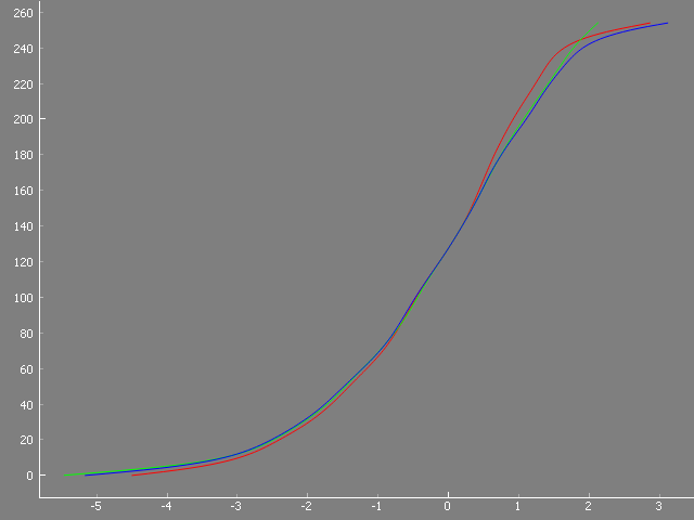
Well, ideally, you want to use only the more or less linear part in the gain curve of your camera, in the case below from -2 EV to about 1 EV for scanning. Your image will more or less mirror the original contrast of your frame, nothing gets squished. That is a working range of about 3-4 EVs.

Now, a difference of 3 EV is not enough for scanning color-reversal film. From experience, I think the range of EVs you are dealing with color-reversal film is between 7-9 EVs, depending on the quality of the film stock and the exposure situation. If you you want to capture such a huge dynamic range, you will need to capture several different exposures from a single frame. (The above gain curve is actually the gain curve of the HQ camera, by the way.)

Assuming for the moment that covering 7 EVs is enough (and for various reasons, that is a quite valid assumption), you would be actually fine to capture just two exposures. I have seen people doing just that. The results are fine, but if you look closely at their results, you notice often some faint banding in the areas where the exposure fusion switched from one exposure to the other one.

So, of course, three exposures are even better. And in fact, I have done quite some scans with only three exposures, utilzing a constant LED source and different exposure times. In this case, I spaced the different exposures larger apart, from 1.5 EVs to 2.5 EVs in order to scan as much of the exposure range as possible.

Now, why do I capture currently with five exposures? Well, there are several reasons. Most importantly, a small patch captured perfectly in one exposure is also captured quite decently in the two neighboring exposures. In a finely tuned exposure fusion algorithm, this leads to a reduction of the camera’s noise level, as more information is available and averaged during the calculation this specific pixel. And with my exposure settings (exposure time = 1/32 sec, digital gain = 1.0, analog gain = 1.2, mode 3) the camera is noisy on the pixel level…

Also, the risk of banding is greatly reduced because for most of the image area, the pixel’s output is an average of at least three exposures.

Finally, I just was not satisfied with the image definition I could achieve in the dark areas of the image - I wanted some headroom here for color grading purposes. Both ends of the density spectrum of the film are recorded only by a single exposure - namely the brightest and the darkest exposure in your exposure stack. While with color-reversal film the highlights are not too challenging, as the original film response curve flattens out here anyway, color-reversal film has a rich image structure in the dark parts of the image.

That is the reason I added additional exposures to get more information from the darker parts of the frame - see below…

Well, that’s simple. My naming of the different exposures simply reflects the purposes of the exposures. Here’s the full list:

  1. Highlight Scan: the purpose of this scan is actually to reproduce even the brightest image parts of the frame. Because of this, the exposure for this scan is chosen in such a way that the brightest image areas stay in value below the flat shoulder in the above pictured gain curve. Indeed, if you look at the highlight scan posted above, you can use a color picker in the perforation hole to check: the 8 bit values of each color channel should be in the range of 240 to 250. Of course, the brightest highlight in the actual frame cannot be brighter than the light source itself - so any highlight contained in the frame will be captured faithfully, without saturation of the scanner’s sensor, in the highlight scan.
  2. Prime Scan: this scan is a little brighter (+1 EV) than the highlight scan, so any real highlight in the original frame is burned out in this scan. However, generally this +1EV-scan delivers sufficient image details in most of the image area and that’s why I call it the “Prime Scan”. This scan turns also out to be the most similar to the output result of the exposure fusion algorithm.
  3. Shadow Scan 00:
  4. Shadow Scan 01:
  5. Shadow Scan 02: - all these scans get brighter and brighter in appearance. Their sole purpose is to record as much shadow detail as possible. Since the film emulsion of color-reversal stock goes very deep into the shadows, there is a lot of recoverable detail hidden here. (Note that this is not the case with the burned out highlights - there is no chance of recovering detail lost due to a too bright film exposure. That’s the reason only one highlight scan is present, in contrast to three different shadow scans.)

I hope this makes my naming of the different exposures a little bit more transparent. Some additional information on how I capture frames can be found here and in the posts following this entry. You will note that I never adjust my scanner’s exposure values to the film stock I am scanning - they are referenced to the maximal output the LED light can achieve and stay constant, whatever footage or film stock I am scanning.

Well, no, I am not confused. And yes, I do use mode 3, which indeed has a native resolution of 4056 x 3040 px. Before I explain, let me give you some numbers (this is a Raspberry Pi 4 as server, connected via LAN with a Win10 PC):

  • Scan Resolution 4056 x 3040 px, (mode 3): 4 fps in live preview, using a LAN-bandwidth of 200 MB/sec. Scan time (5 exposures) for a single frame: 3.5 sec
  • Scan Resolution 2028 x 1520 px (scaled down from 4056x3040px , mode 3): 10 fps in live preview, using a LAN-bandwidth of 155 MB/sec. Scan time (5 exposures) for a single frame: 2.3 sec

So: I am using the HQ camera in mode 3, but let the camera scale down the original image to a lower resolution. That gives me a temporal advantage of about 1.2 sec per scanned frame, reducing overall scan time for a larger film project (40000 frames → more than half a day).

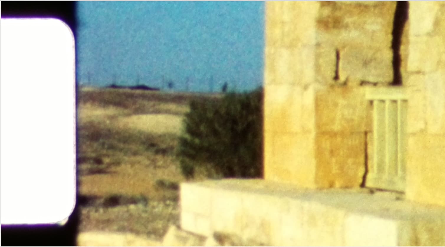
Here’s a comparision between the image quality obtained with the full-scale 4056 x 3040 px resolution of mode 3

and the quality obtained with half that resolution (2028 x 1520 px, mode 3)

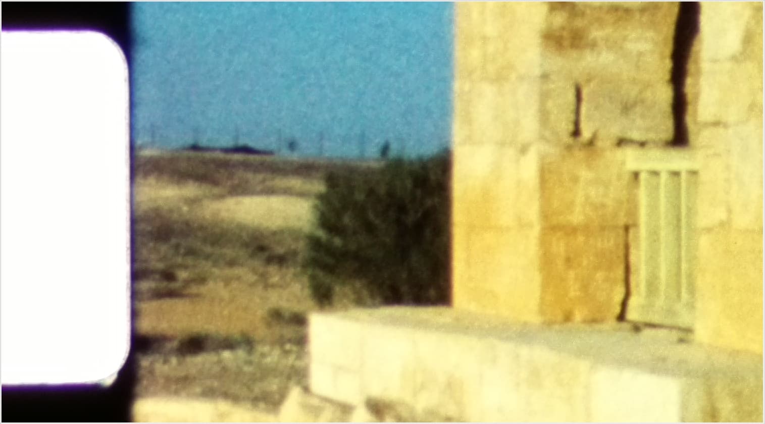
For my taste, the drop in image quality is not so noticeable that it warrants the additional +1 sec delay for each frame scan.

Well, I have uploaded the exposure fusion result of two scenes I used above in the original resolution, but as an encoded video file. The original data would just be too large to store it somewhere (I also have a rather slow internet connection). Anyway, this here should be the download link.

1 Like

I wanted to see if Final Cut Pro could stabilize the images better.
But when I play the downloaded file on my 17" iMac in the QuickTime Player, I keep getting really weird artifacts at the same frames.

@Hans: … interesting. Nice filter effect! :upside_down_face:

Well, I do not know what happened here. This file was created in daVinici Resolve Studio v17.1.0.0024 with the following settings:

I downloaded the file again and played it successfully in VLC and VirtualDub on my Win10-PC…

Must be some codec misinterpretation; actually, I wanted to upload for @dgalland the raw frames, but living in Germany I only have a 1.8 Mbit/sec internet line, so that was no option for me. Besides, I do not have that much internet space available anyway.

Well, if anybody has better video encoding settings, I am happy to retry it again.

The only difference I can see in the settings is that you have an encoder option. This option is missing on the Mac version of DaVinci Resolve (Studio).
I’m curious what options you have here except NVIDIA.

there are just two options: “NVIDIA” and “Native”. The “Native” option features less settings:

and encoding time doubles approximately, compared to the “NVIDIA” option. File size is only 50MB, compared to the “NVIDIA” rendering which comes to approximately 150MB.

It gets crazier when I import the clip into Final Cut Pro.

  1. There are multiple black frames in the timeline and the artifacts are the same as in the QuickTime Player
  2. Background rendering goes wild, keeps starting and stopping
  3. The viewer thinks it is some kind of cinemascope format but the inspector gives the correct format
  4. When the image is masked out, you see that the white balance is not correct and there is still a lot that can be corrected in the shadows and highlights

hmmm… - there exists a VLC version for Mac OS X. You might want to install this player and check how it is doing with the video file in question. Again, I downloaded my own video file and tested it with WIN10 software, namely VirtualDub and VLC (for Windows). Everything worked fine…

I am neither a Mac user nor a Final Cut Pro user; however with Windows-software, you often ran into troubles between incompatible DirectShow-codecs, sometimes left over from some old installation. Again, this video file was specifically prepared for @dgalland to try out his avisynth-scripts, and he has not yet said anything on how the video file works for him. Nor has anybody else noted any issues. Frankly, I do not know how to solve this issue…

well, that’s no bug but a feature! This is the raw footage as it came out of my scanner/exposure fusion software. It is not color-corrected at this point in the processing pipeline on purpose. I am doing color-correction as the very last step of the editing process.

Note the histograms reveal that only a part of the full dynamic range of the frames are used - this is done on purpose, to be sure that during post processing work no clipping of data can accidentally happen. That “there is still a lot that can be corrected in the shadows and highlights” is actually the whole purpose of my scanner/software design. :innocent:

Would it be helpful for you if I try to re-encode the file in a more standard format, like 1920x1080 px and adjust a little bit the image intensities?

No thanks, I just wanted to test the stabilization using the punch hole in Final Cut Pro and/or DaVinci Resolve Studio. But your clip doesn’t play smoothly in either program.

Oddly enough, it just plays in Adobe Premiere Pro.

@Hans: just out of curiousity, I downloaded the clip again (just to be sure that Dropbox didn’t recode) and stuffed it in my DaVinci Resolve - guess what, no problems playing the file at all on my Win10 station.

Tested again with all programs I could find on my PC: VirtualDub, VLC, DaVinci Resolve, Magix Video deluxe Plus 20.0.1.80 and finally the Windows Media Player (current and “classic” (the later from 2011)). The video file worked with all these software.

Maybe the video stream settings of this file are a little bit too much off with respect to the standard ones. This video file was encoded at a resolution of 2016x1512 px and a frame rate of 18 fps. Not the usual 1920x1080 px @ 24 fps.

Also, in the video file which you have trouble decoding, the sprocket hole has already been stabilized.

So here’s a better example: I have encoded with 1920x1080 @ 18 fps (which should be closer to the standard) the raw prime scan of this footage (at a lower 1920x1080 resolution), which is a much more challenging footage for sprocket stabilization. Have a look at Example Scene 03-04 LDR01 raw.mov and see how this works in your setup.

@cpixip
I’m using Final Cut Pro even before Apple officially announced it, even had to sign a Non Disclosure for it.
The size of the format will not be the problem, I also edit with 8K Apple ProRes RAW. And Final Cut Pro is one of the few NLEs where you can place all formats, fps and codecs in one timeline and play and export everything perfectly.

The reason that the clip now plays properly will not be the format, but the encoding.
The first version was AVC (High@L5) (Cabac / 2 Ref FRames) and the second AVC (Main@L4) (2 Ref frames) encoded.

And it is indeed surprising how well Final Cut Pro stabilizes the images. You certainly don’t have to come up with another difficult solution such as LED, laser or OpenCV.

Thanks.

:+1: fine that this worked!

A further update. Recapped my old own work on motion estimation (neural network stuff, but in the 1990’s), read about the current state of the art (mainly neural network stuff utilizing GPUs) and digged further into the avisynth-motion estimation stuff. (The goal is: can we improve the visual quality of raw scans of old Super-8 footage? It follows a path initially started with VideoFred’s (Freddy Van de Putte) avisynth scripts, with a lot of people coming up with own versions.)

The avisynth motion estimation stuff is mainly based on classical algorithms, very much similar to what is used in video-encoding like h.264 and the like. Lots of rather undocumented parameters to play with.

The new neural network stuff looks promising, but has two disadvantages. First, work is focused on video material, and analog film is quite a different beast. So at least a retraining would be necessary for film stock. Not sure how these approached would perform on challenging film grain like the one present in small format films.

Another point is that example implementations of these new neural network stuff are often based on specific programming environments, in this case mostly piTorch, which in turn requires specific hardware to achieve a decent performance. That’s a plan for the next year.

So in the meantime I dug futher into the parameter hell of avisynth’s motion estimation engine and could improve the behaviour of this algorithm with respect to film grain. Here’s an example, using my favorite test clip.

In order to isolate the effect of the film grain on the improvement process, I stabilized the footage in daVinci Resolve before running the algorithm. A cut-out of the original scans (displayed for reference in the lower left) shows that the source (KodaChrome 40) is noisy all over the place, even in well-exposed areas. As expected, the noise gets worse in the darker image areas (this is due to the way these color-reversal films were engineered). Both the amplitude as well as the spatial extent increase. To the right, the same cut-out is shown after processing. There is still “pixel dancing” visible, no question, but the situation is improved from the results presented at the start of this thread. The recovery of structure especially in the darker areas of the source is quite noticable. Note that this is exposure-fused material (5 exposures into one) - the dark areas in this footage would be nearly black in the best overall single exposure.

So, in summary, it seems possible to recover image information from grainy Super-8 material beyond what is usually visible in a normal scan. I have other film stock (like Agfachrome and Fuji) which have even more film grain than Kodachrome and I have not yet tested these. However, for my goal resolution of 960 x 720 px, the results with Kodachrome stock are already usable.

2 Likes

That’s remarkable.
I do see a bit of dancing blocks, not sure if it is vimeo. But the improvement of the noise/details is remarkable.

:smile: - well, this is probably not vimeo, in this case!

I am still searching for the right settings, which is challenging within the avisynth environment. I can only guess the impact of most parameters available in the motion-estimation engine. They are basically not documented.

At this point in time, I am using the avisynth stuff to give me an idea on what might be possible; if the improvements possible validate further developement, I think in the end I will roll my own software so that I know what the different parameter are doing.

In the example above, I needed to cheat slightly - in order to make the pixel dancing visible, I had to stabilize the footage. Since after stabilization, the scene was mostly static (if you look closely, you see a slight perspective shift), the result above is very similar what super-resolution algorithms would achieve - given that the motion estimation was perfect. Of course, the motion estimation gets fooled by the film grain, and that is what I wanted to test.

Now, additional challenges to motion estimations are also large movements in the scene, as well as scene changes itself. The later introduces one or two initial frames where not enough data is available for the faithful reconstruct of these frames. So in restored scenes, you might notice a little pumping of quality between scene cuts. One way to get rid of this is of course to cut away the very first and last frame of each sequence, which is most of the time no big deal.

Much more challenging are fast and large motions within a scene. Here, chances are that the motion estimation fails, leading to visual artefacts. Yet other challenges lurk: one has to do with thin, elongated objects (they tend to be overlooked by motion estimation algorithms), the other with transparent objects (up to my knowledge, not motion estimation algorithm can handle this yet).

Whether the errors in the motion estimation are noticable or not depends on a number of things, most notably on the original content of the scene. In the end, it’s the viewer who decides. My current challenge is to test various parameter sets on various scenes in the hope to find a generic, balanced set of parameters which works with most material.

In this respect, here are current enhancment results of two scenes which contain large image motions and huge exposure variations. It’s from a 1981 Kodachrome movie, taken with a different Super-8 camera and a different scanning camera than the clip discussed above.

On the left is the original 5 exposure fused scan, on the right the enhanced version. Top-left is the best single exposure scan included for reference. You might want to set the playback quality to the highest setting and even reduce the playback speed to 0.5 for this one, as the movements are quite fast. Therefore, here’s an additional framegrab

The improvement is not so visible as in the previous example, but the difference between left and right image is quite noticable in man in the foreground. At least in this example which was processed with the same parameters as the clip posted above from Jordan, I am actually ok with the results so far.If you look closely at the very last frames of the first scene, you will notice some strong artefacts, due to the failling motion estimation there. However, when the sequence is run at the normal 18 fps, it’s hardly noticable.

Thank you for the complete explanation.
In the latest clip I could not see the same blocks, perhaps because of the movement. The improvements are noticeable and certainly worthwhile the effort.
A couple of observations.

  • In the latest clip what I do see is a flash of grain on the blue sky (upper left side) second 5 or 6.
  • Some of the very fine detail embedded in the noise is taken away. In the still there are faint powerlines visible, and in the bicycle wheel lines.

Understand this is a compromise between enhancement, denoising, and perceived quality. The above observations are certainly a good trade-off for the improved picture.

In regards to the previous clip, I noticed that the dancing blocks are more apparent in the dark areas. I played the click at 1080 at 0.5 speed.

I think one clue may be that due to the stacking, the resulting image would have different noise profiles in different areas, which would make it very difficult to have a setup to catch all. One way to confirm that hypothesis would be to apply your process on each exposure separately, and finalize with the stacking. That may not be practical for a final solution (for the times fold processing) but at least it would help you on locating the source. That is also apparent on the second clip where the noise ‘visibility’ is inversely proportional to the luminance of the area. Clear areas are clean, and noise increases with lower luminance.

If I understood correctly, the current process order is 1-stacking/merging 2-Davinci 3- Avisynth. The test to check the hypotheses could be 1- stabilize each exposure, 2 Avisynth to each exposure, 3- stack/merge.

One additional consideration, in the above you may have different noise profiles for each of the exposure tracks.

It is a bit of a rabbit hole, but it would help you understand the issue. Hope it helps.