Kodachrome Colors

[cpixip]

@npiegdon

I wouldn’t solve the kind of discrepancy you pointed out in the gray swatch by boosting the whole channel uniformly. Instead, I’d solve it with a calibrated 3D LUT. That’s exactly what that particular tool is for and it defeats the problem perfectly.

Yep, exactly. Besides, it might not even be noticable in the first place. Variances in the development process in those old days might have a much larger influence on color fidelity than this.

@npiegdon

Kodachrome calibration targets are no longer available, which makes me wonder how far off any target printed using a three-dye system would be vs. a Kodachrome target. Certainly, every three-dye film stock will exhibit the same wavy characteristics for the same reasons that Kodachrome does. So, if the same dye curves are available for other stocks, I’d be curious to see how far off they were from one another. More specifically: my calibrated 3D LUT comes from an Ektachrome target with 288 swatches. How far off would some hypothetical simulated Ektachrome curves be from your simulated Kodachrome curves?

Interesting question. Here’s a plot of the digitized data from the Kodachrome 25 data sheet,

and here’s the equivalent one for Ektachrome 100D:

Comparing the dye’s spectra separately, one gets for the yellow dyes:

This is the comparision for the magenta ones:

and finally for the cyan dyes:

There is indeed not too much difference how the dye spectra behave over the interesting wavelength range.

@npiegdon

Another detail: it’s useful to remember we’re not taking point samples on these curves. “Narrowband”–at least, until you’re using lasers or adding bandpass filters–isn’t necessarily as narrow as it sounds. Recall my measurements where each LED had a bandwidth between 30 to 40nm. Taking the extra bandwidth into account doesn’t solve the problem, but it would soften it a bit on average.

Some commercial scanners do use rather narrow interference-based bandpass filters. I am more interested on whether the Swiss setup (described in the DIASTOR-paper) does make any sense. Frankly, I think not. Here are some illumination spectra I generally play around with:

You might be interested in the yellow curve. Comparing this to the Swiss illumination choice, it’s obvious that your narrowband setup delivers power on all wavelengths. The Swiss illumination (if I used the correct numbers - need to check this again) has however an annoying dip between 610 nm and 620 nm. In other words: basically features a blind spot. No 3D-LUT can recover from this.

I do not think that this issue is too crucial, given the broad dye spectra, but this is exactly what I am interested in.

Certainly the scan quality depends on the placement of the three narrowband LEDs - that’s what I discovered when I started to look into film scanning. My original setup was very similar to the Swiss one, a later one more like your own setup, yielding better results.

[cpixip]

@npiegdon

So, if the same dye curves are available for other stocks, I’d be curious to see how far off they were from one another. More specifically: my calibrated 3D LUT comes from an Ektachrome target with 288 swatches. How far off would some hypothetical simulated Ektachrome curves be from your simulated Kodachrome curves?

Update: (let’s see how many graphs I can pack into a single post): here is the data comparing Kodachrome 25 vs Ektachrome 100D. Remember: using the spectral date of the print dye based spectra of the BabelColor Average data of the colour python package, I numerically calculated the necessary dye densities of a simulated film to match exactly the color of each patch of the BabelColor Average color chart.

The comparison between the simulated data for Kodachrome 25 and the BabelColor Average color chart can be found in one of the posts above. Here’s the simulated Ektachrome color chart:

Again, the numerical procedure was able to match the color impression of the reference color chart exactly within the numerical precision, under D65 illumination.

So how do the different spectra of each patch compare to each other? Here are the graphs:

While the print dyes vary rather smoothly and are close to the ideal horizontal line in the case of neutral patches, both spectra created by film dyes show a little waviness - Kodachrome 25 more than Ektachrome 100D.

Remember that at both ends of the spectrum deviations between the spectra will only have a minor effect on the perceived color, as the human visual system is mostly insensitive in these spectral ranges.

[npiegdon]

@cpixip

You might be interested in the yellow curve.

Haha, I am! This is awesome. What a fast turn-around time. There is so much data here! Thanks for all your effort.

The cyan dye isn’t as close between the two film stocks as I would have liked. So–with my 660nm deep red LED in mind–patches like orange[6] and moderate red[8] have larger discrepancies than I was hoping to see.

I wonder… with a real, measured Ekta target, and this simulated difference between the two, would it be possible to combine them into a simulated Kodachrome calibration (not unlike your scientific tuning file)? I’m guessing it would be a little fiddlier and also require the simulation of the lighting setup as one of the inputs, but that would be cool to end up with a “measured” Kodachrome calibration without actually having a calibration target printed on Kodachrome.

Presumably the same could be done for any film stock with published curves like these. The possibilities are pretty exciting!

[cpixip]

@npiegdon

So–with my 660nm deep red LED in mind–patches like orange[6] and moderate red[8] have larger discrepancies than I was hoping to see.

I think we should take these exercises with more than a grain of salt. Citing here a remote sensing paper from 1978 (“A Method of Determining Spectral Analytical Dye Densities”, FL Scarpage & GA Friederichs, v44/10, pp 1293-1301):

So the curves in the data sheets are probably only qualitatively valid. I have at least two different Kodachrome 25 films were a few of the 15 m rolls used in the films display a noticable greenish tint - most probably a mishap during development. Another caveat is the following: as elaborated above, I am not 100% sure that my interpretation of the “Diffuse Spectral Density”-graphs is the correct one.

So I think all of the discussions in this thread are more academic than practical.

Nevertheless: I learned a few things. For example, I learned that there is a difference between a classical color checker printed with carefully selected print dyes (explaining the price!) and a color checker chart created by using only three different film dyes. The latter inevitably leads to a certain ripple in the resulting spectrum. But again, I think this is irrelevant in practice. What I also learned from these simulations is that the gray patches of real color checker actually have a small color cast. They are not really “gray” in a strict sense. One can see this in a cutout near the whitepoint of the CIE-diagram:

While the whitepatch 18 is exactly at the whitepoint of the sRGB space, the darker patches deviate from this position a little bit.

Whether the difference in the dye’s spectra between Kodachrome 25 and Ektachrome 100D make any difference in a scanning situation remains to be seen.To figure this out, one needs to implement a virtual camera that at least somewhat mimics your processing (using an optimized LUT) - my gut feeling is that this small deviation doesn’t matter.

@npiegdon

I wonder… with a real, measured Ekta target, and this simulated difference between the two, would it be possible to combine them into a simulated Kodachrome calibration (not unlike your scientific tuning file)? I’m guessing it would be a little fiddlier and also require the simulation of the lighting setup as one of the inputs, but that would be cool to end up with a “measured” Kodachrome calibration without actually having a calibration target printed on Kodachrome.

Interesting idea - but that would be really hard to achieve, if it is possible at all. One would for sure need to take into account the different sampling of the dye spectra with respect to the different illuminations. And at least in the moment, I have no idea how to approach such a calculation algorithmically. Most likely the correction would be rather small anyway, completely masked by other factors.

Again, these exercises are largely academic. Nowadays, every scan undergoes color correction and grading, in effect replacing every scan, no matter how carefully created, with an image graded according to some personal taste…

In closing, let me cite an old blog-enty by Jim Kasson (photographer and color scientist/2015):

[cpixip]

… ok, time to wrap things up in this thread. My primary goal was to find out what scanner illumination yields better results, narrowband sampling via three differently colored LEDs or wideband sampling via an appropriate whitelight LED.

Remember, these are simulations (which might be wrong) based on old data sheets (where I am not sure I am interpreting the data correctly, or even sure that the data is correct).

Nevertheless, this is what I did:

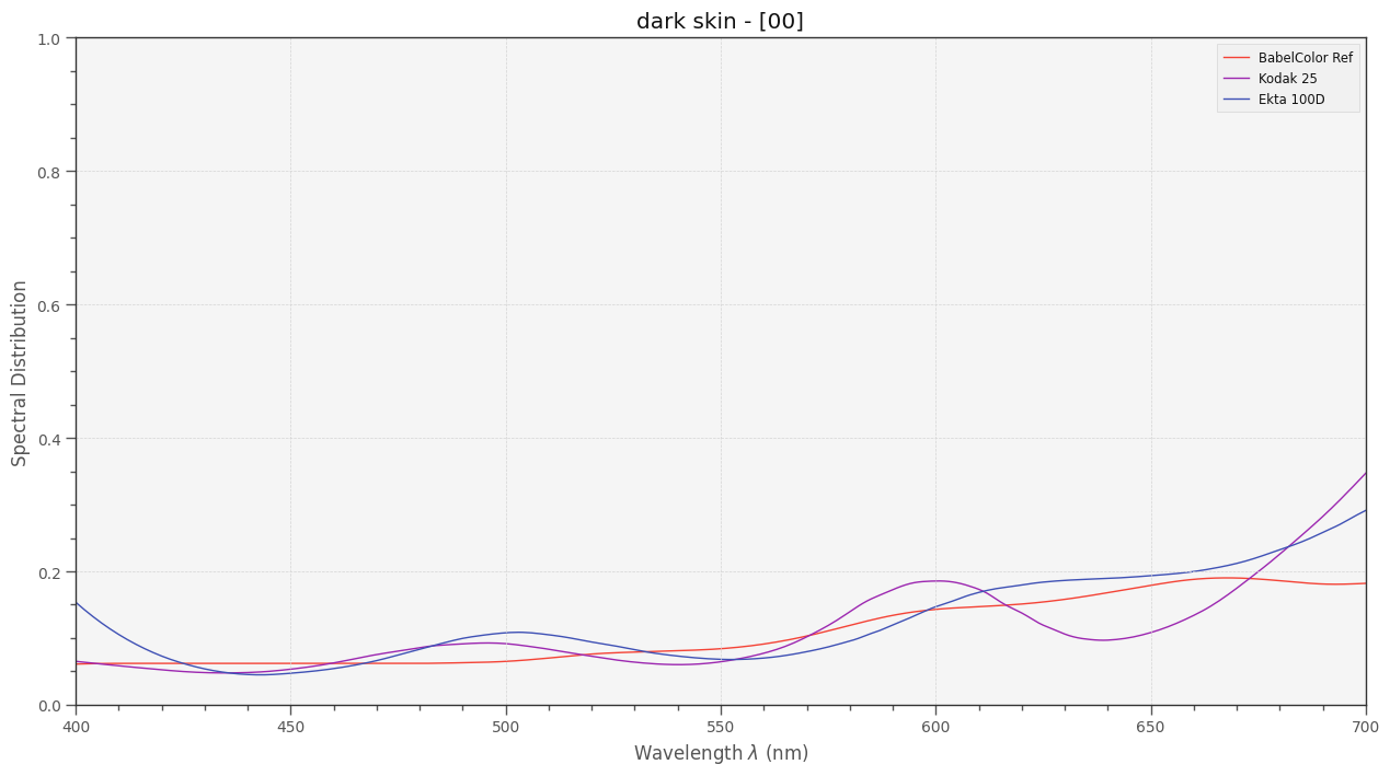
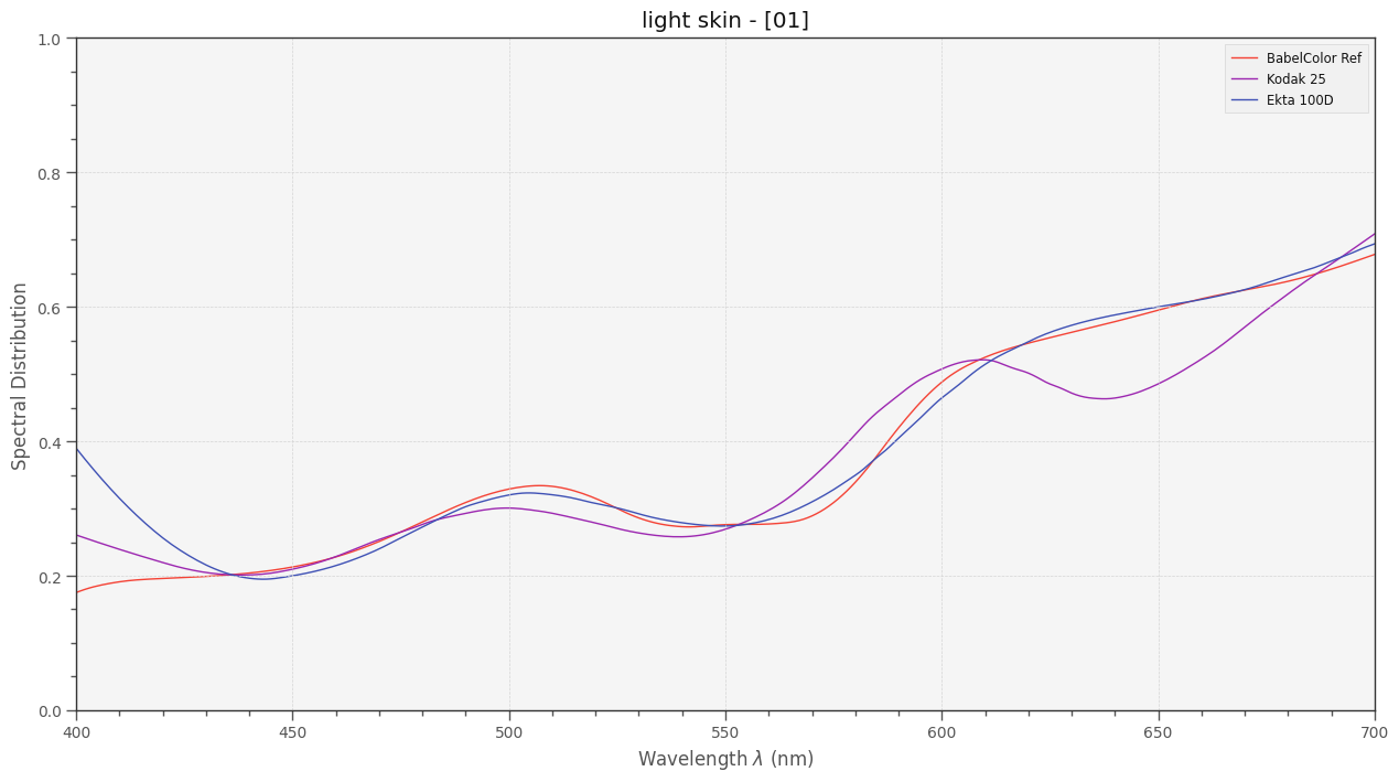
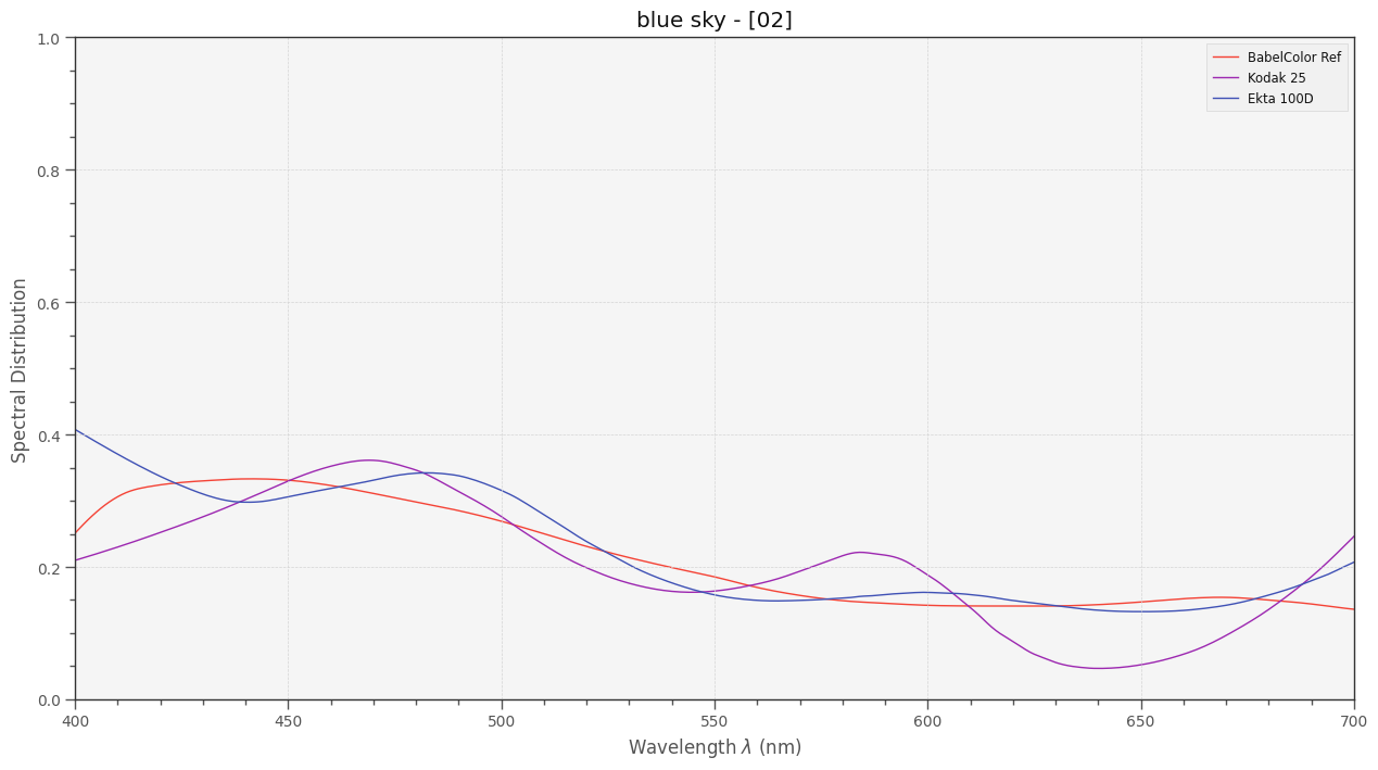
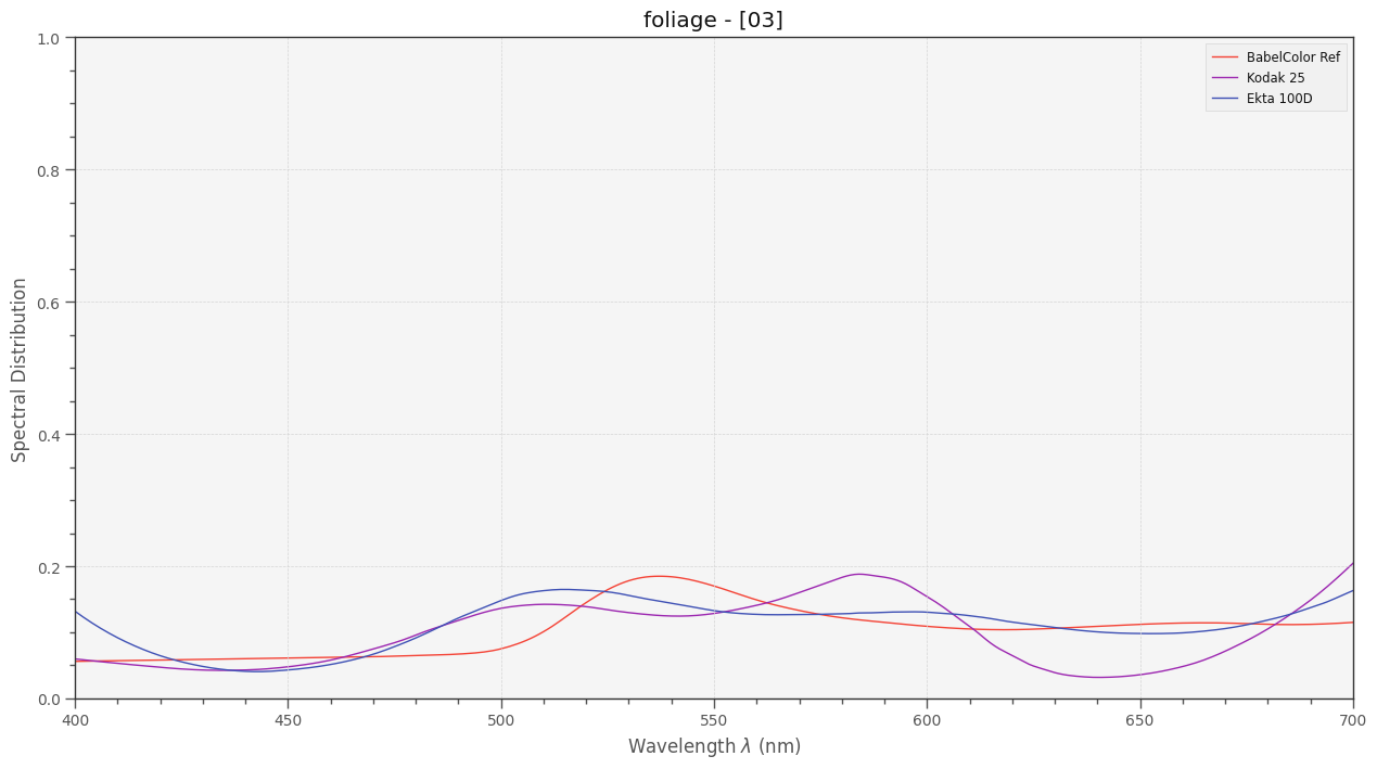
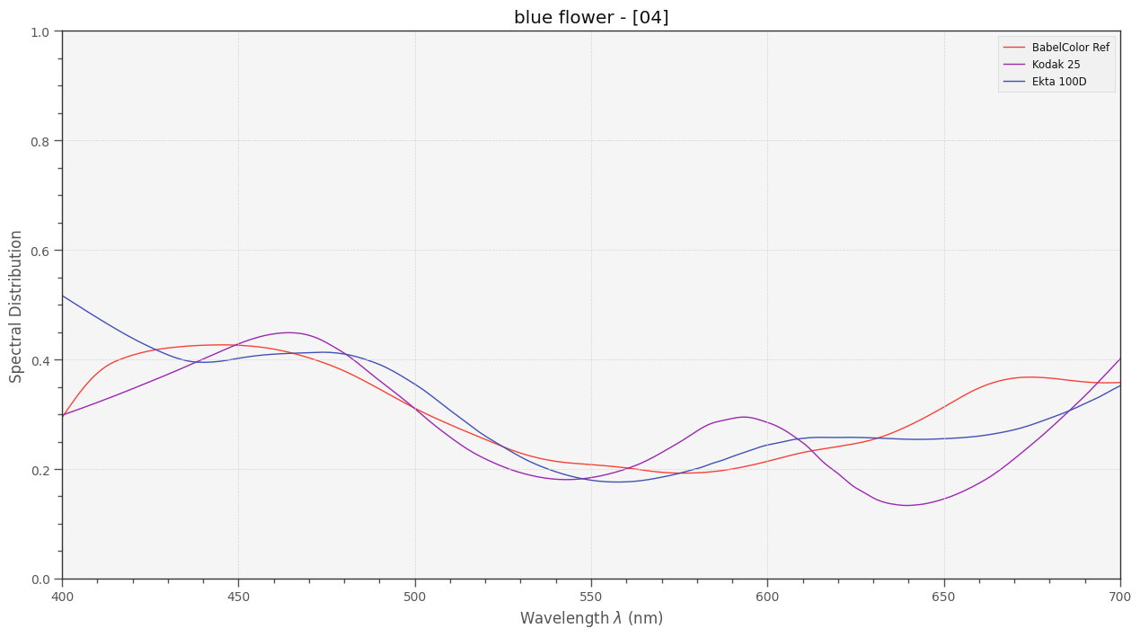
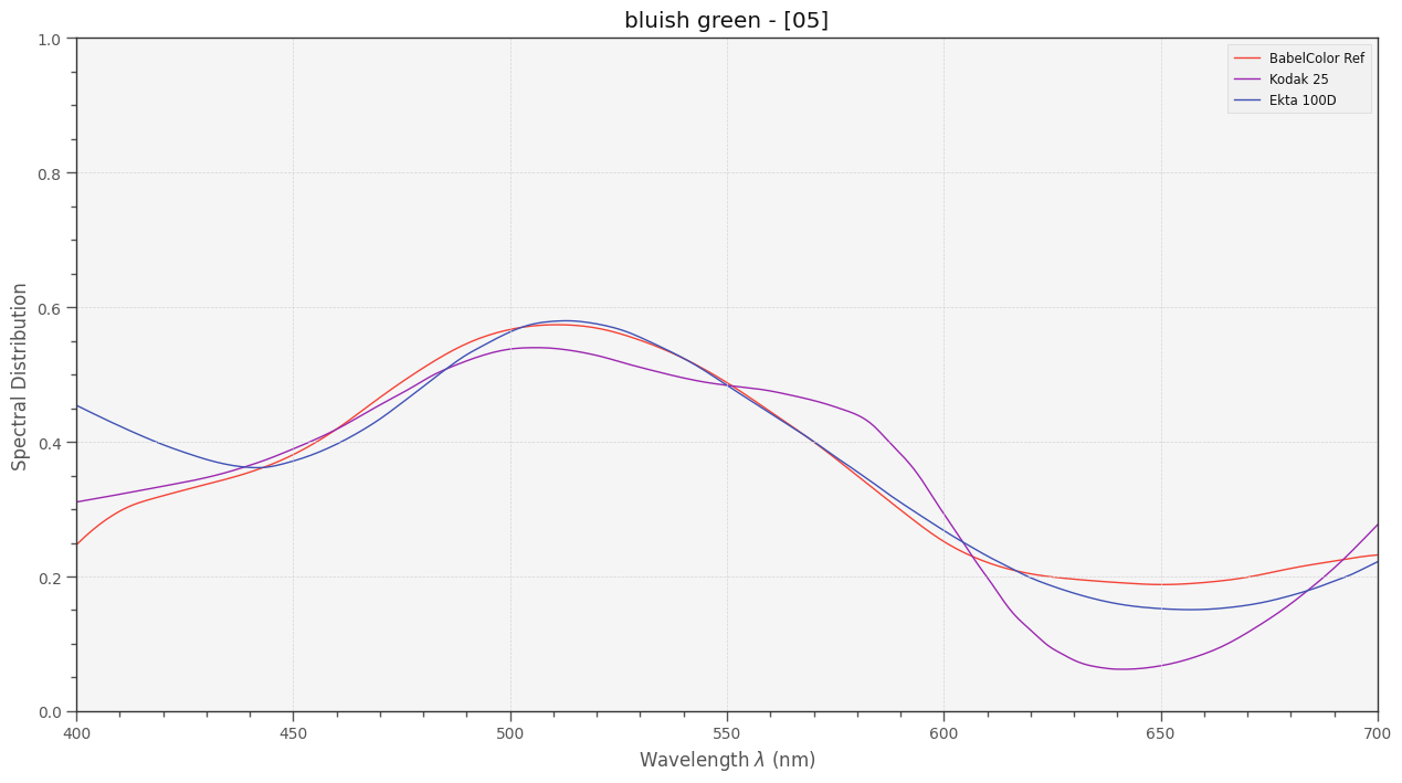
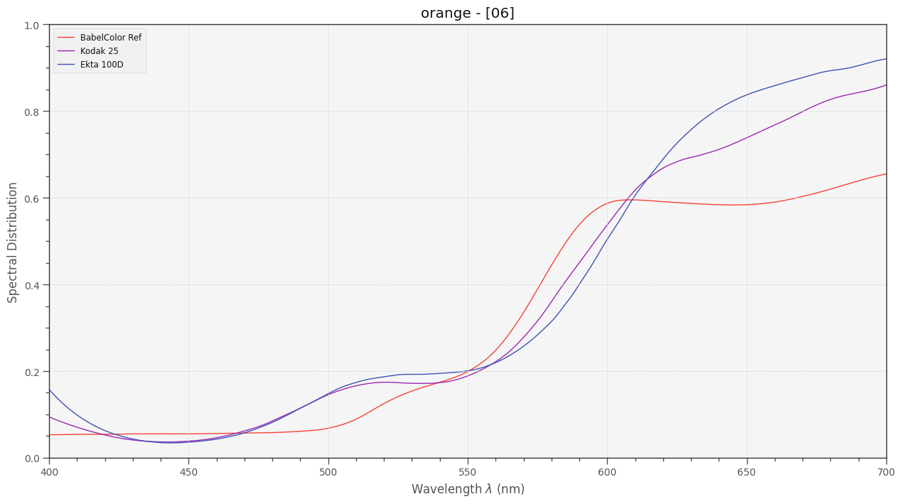
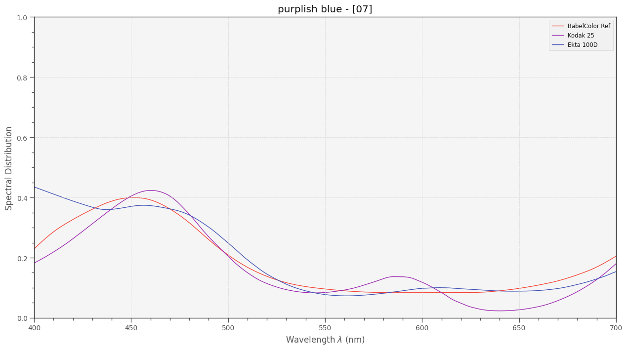
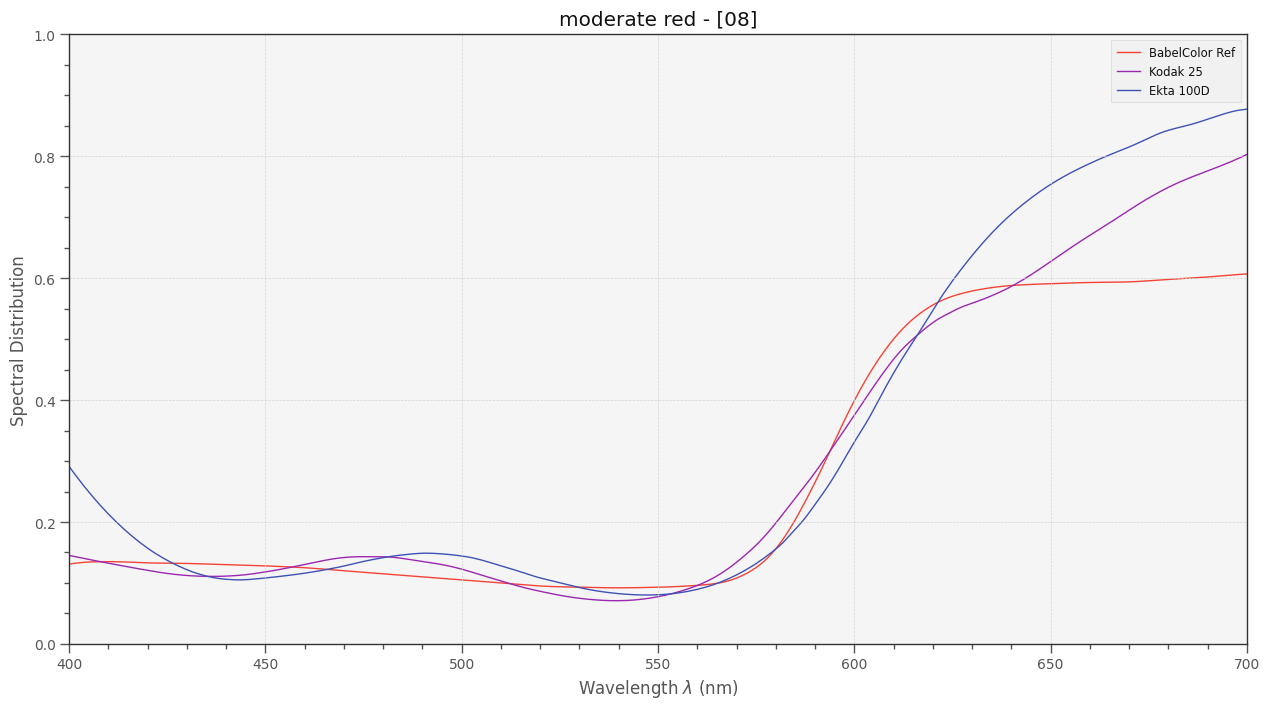
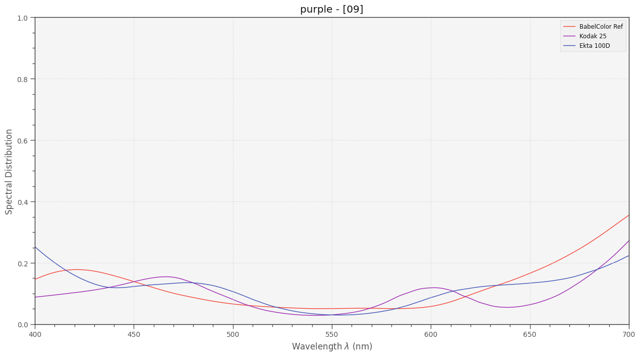
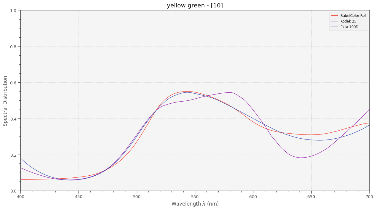
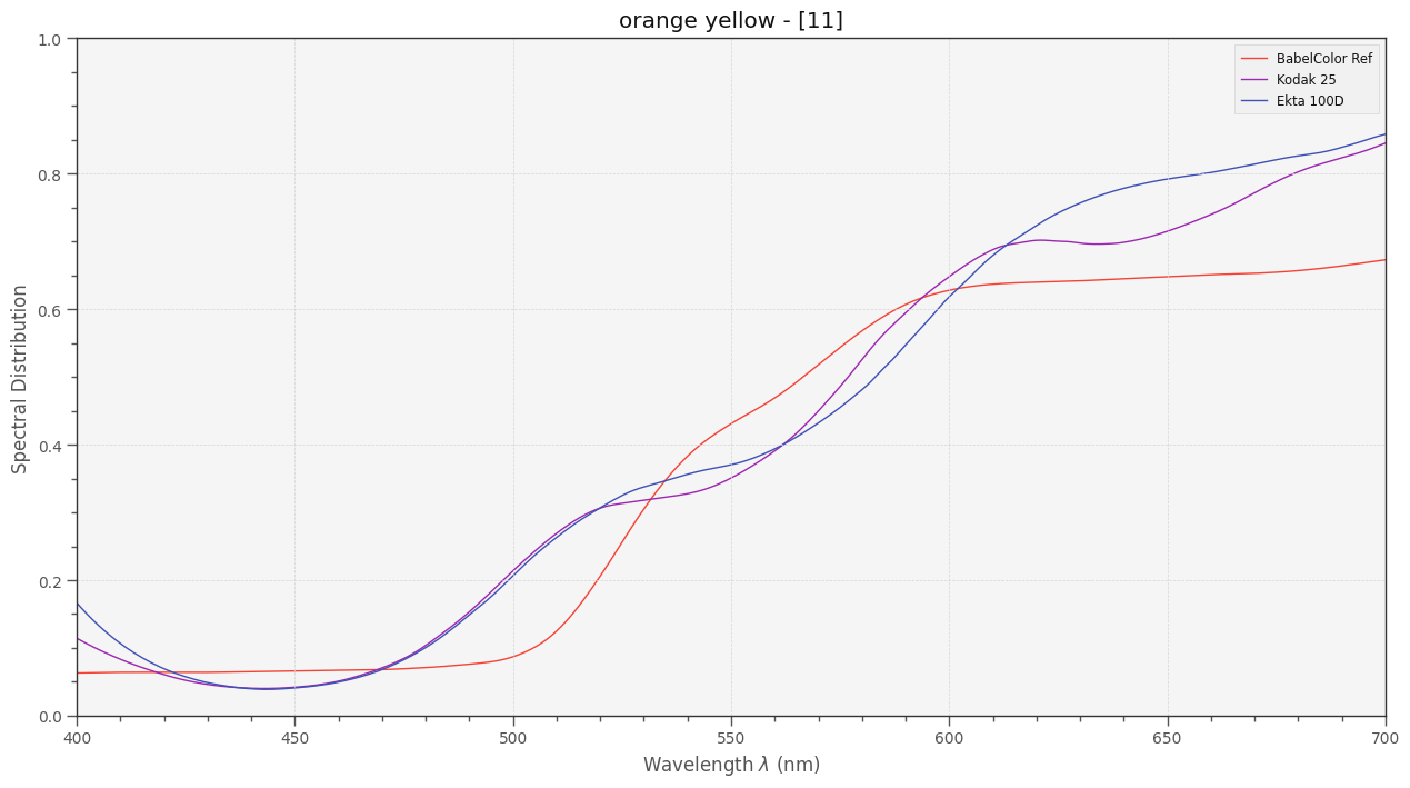
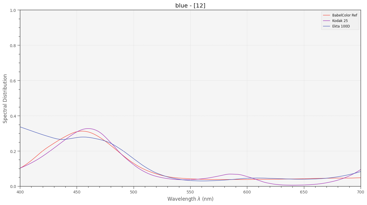
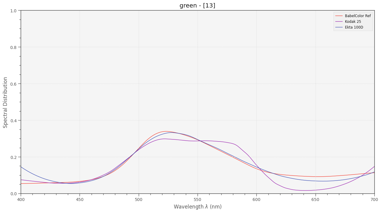
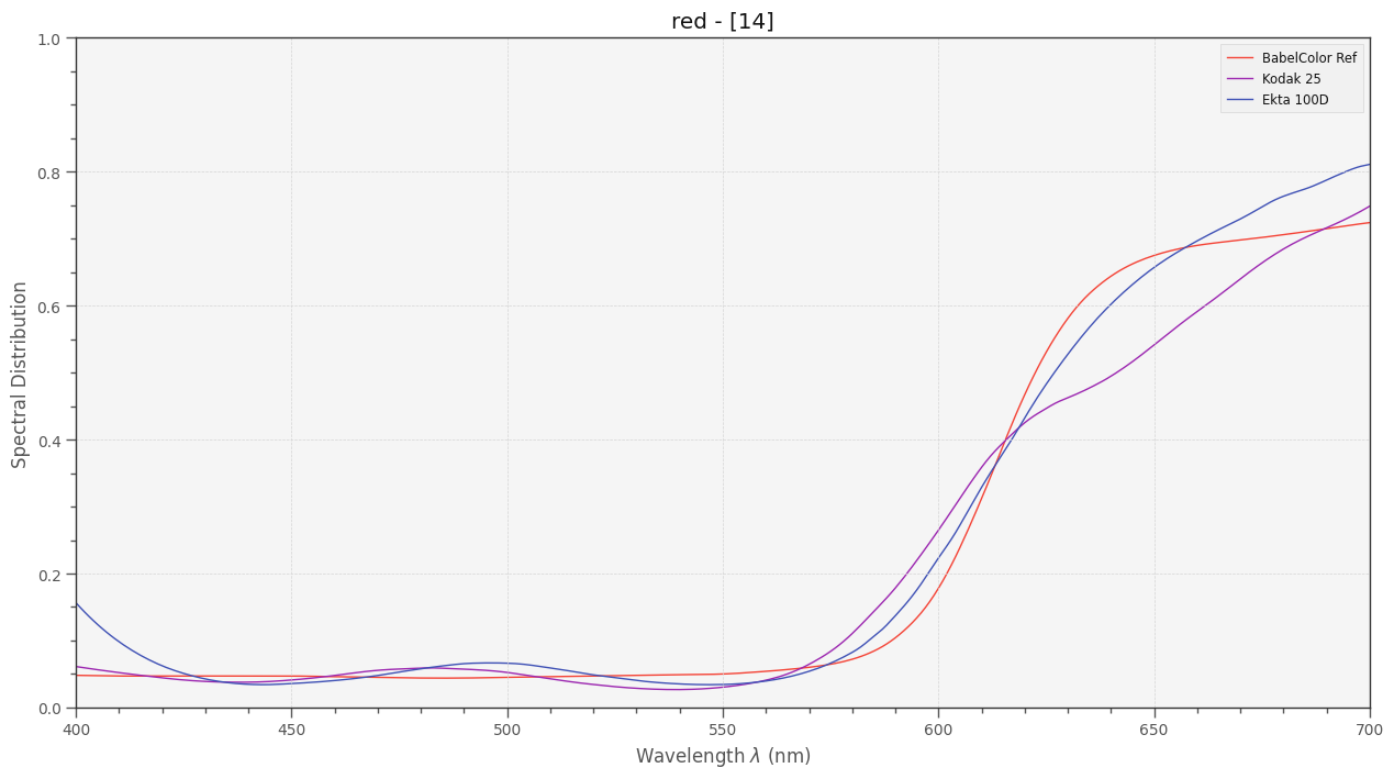
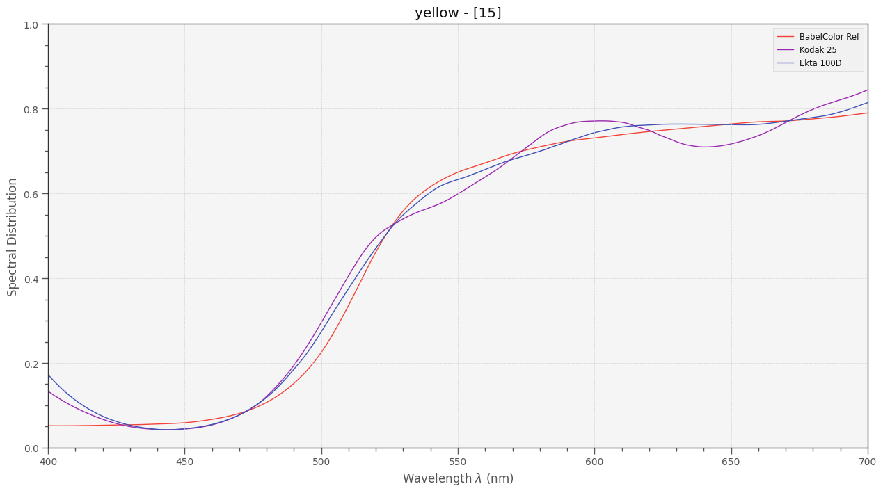
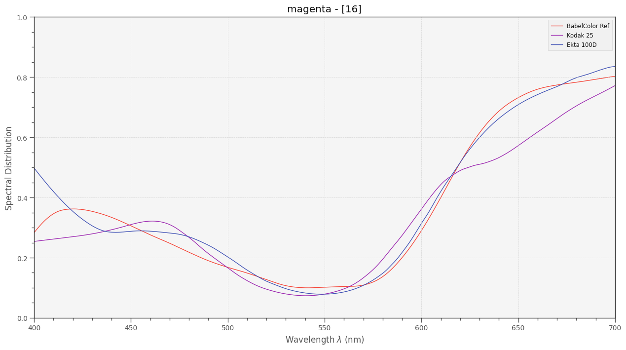
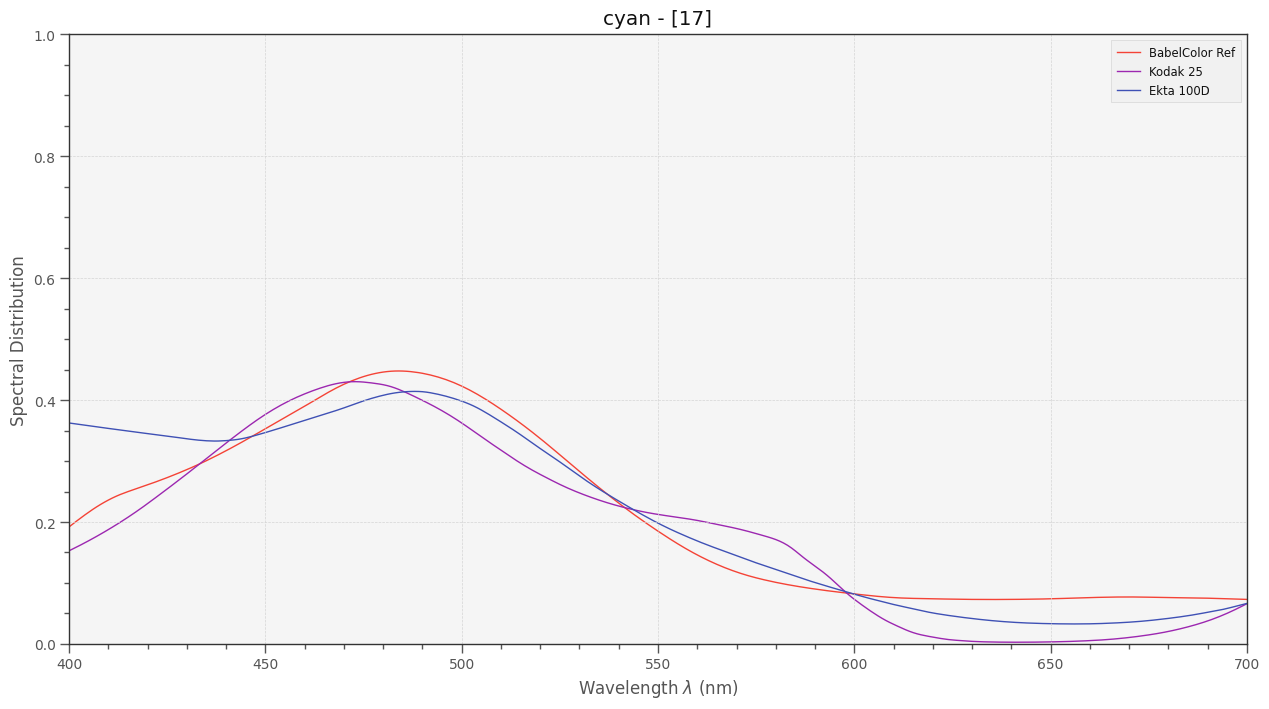
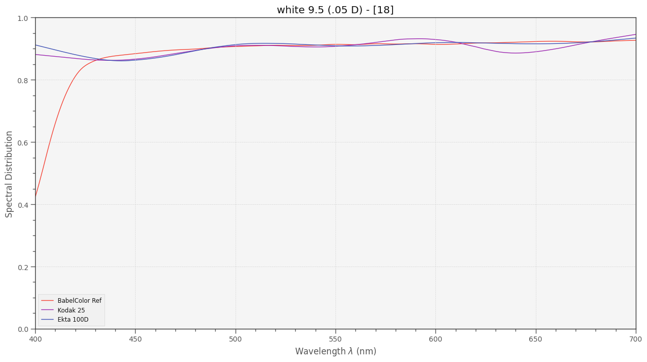
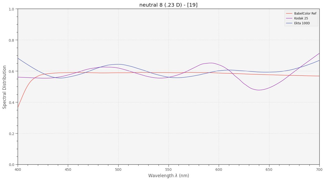
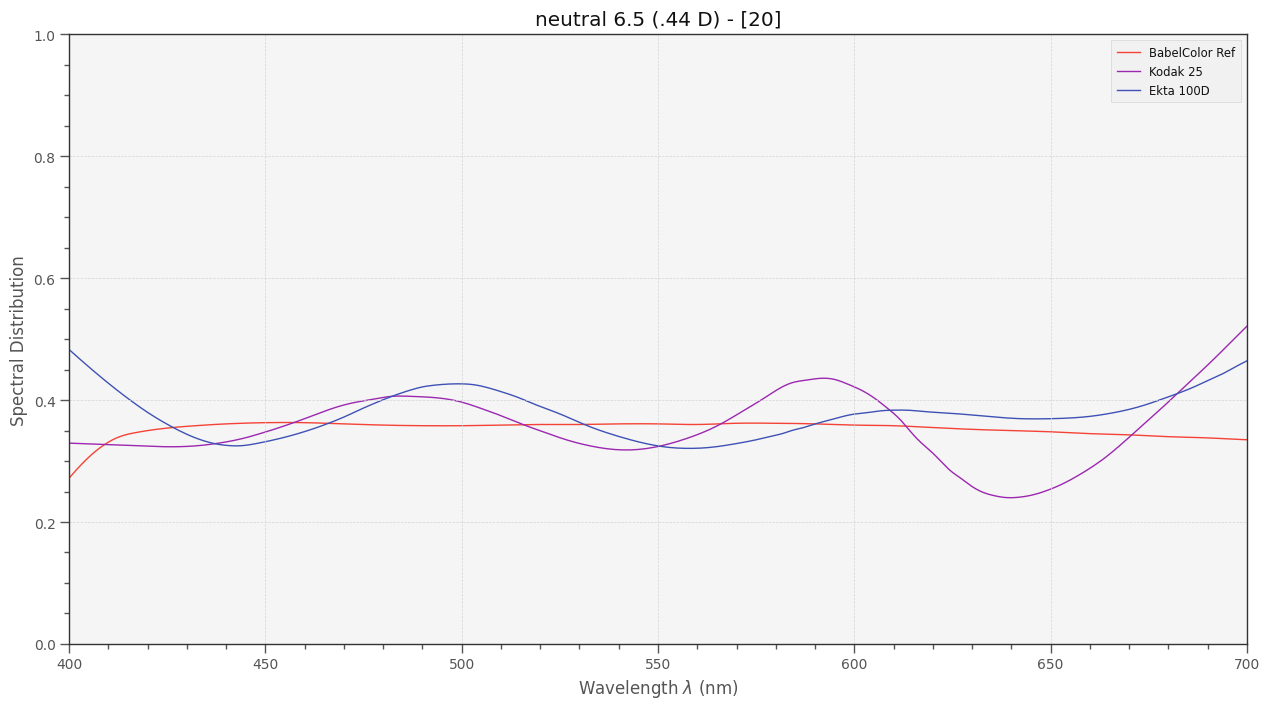
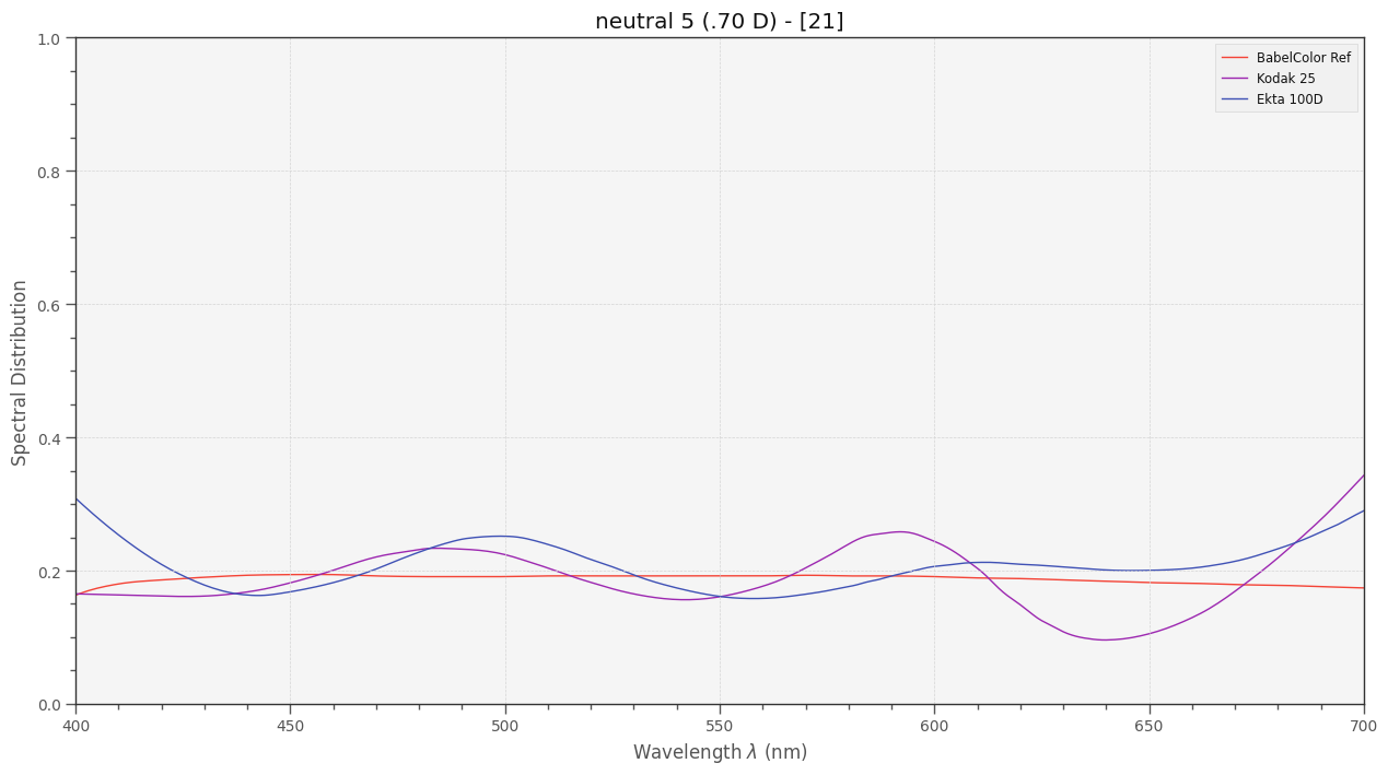
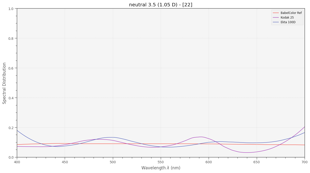
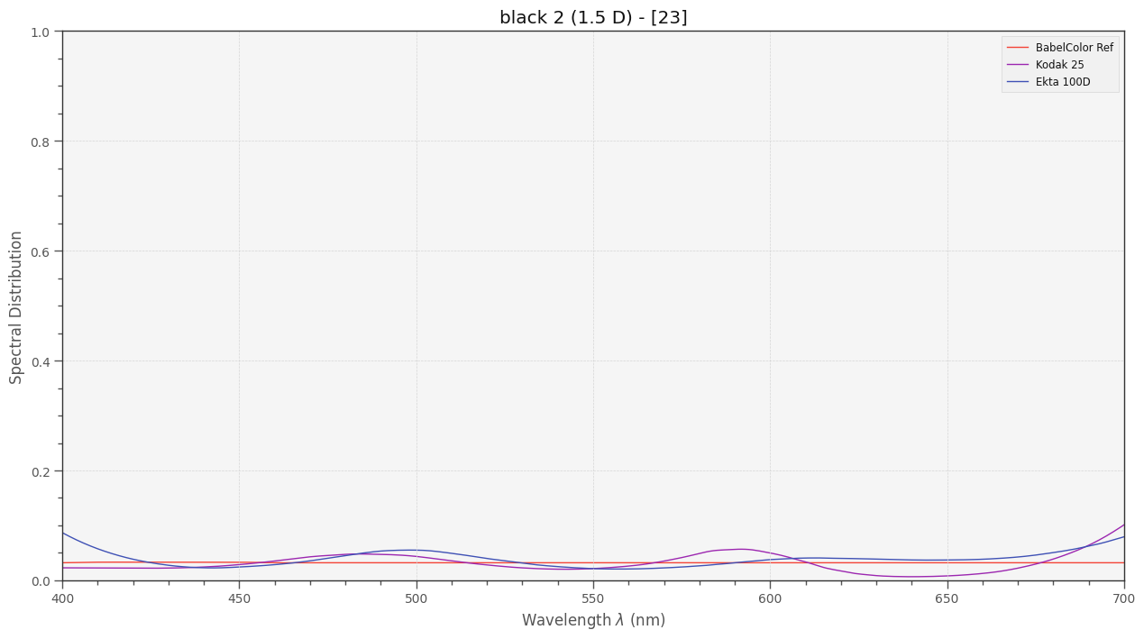
1. Created a virtual color chart based on printed dye spectra for reference (“Ref”).
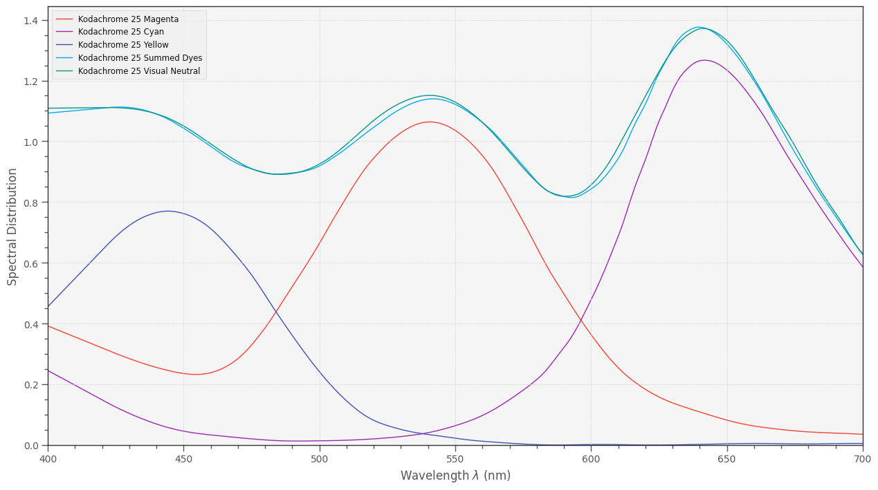
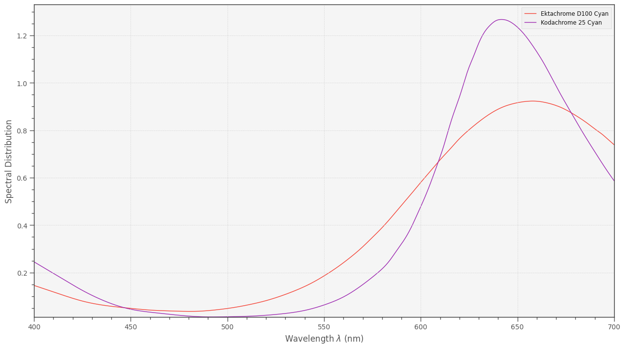
2. Created a second virtual color chart with the same appearance when viewed in D65 illumination, but using only the spectral characteristics of Kodakchrome 25 film (“Kodak”).
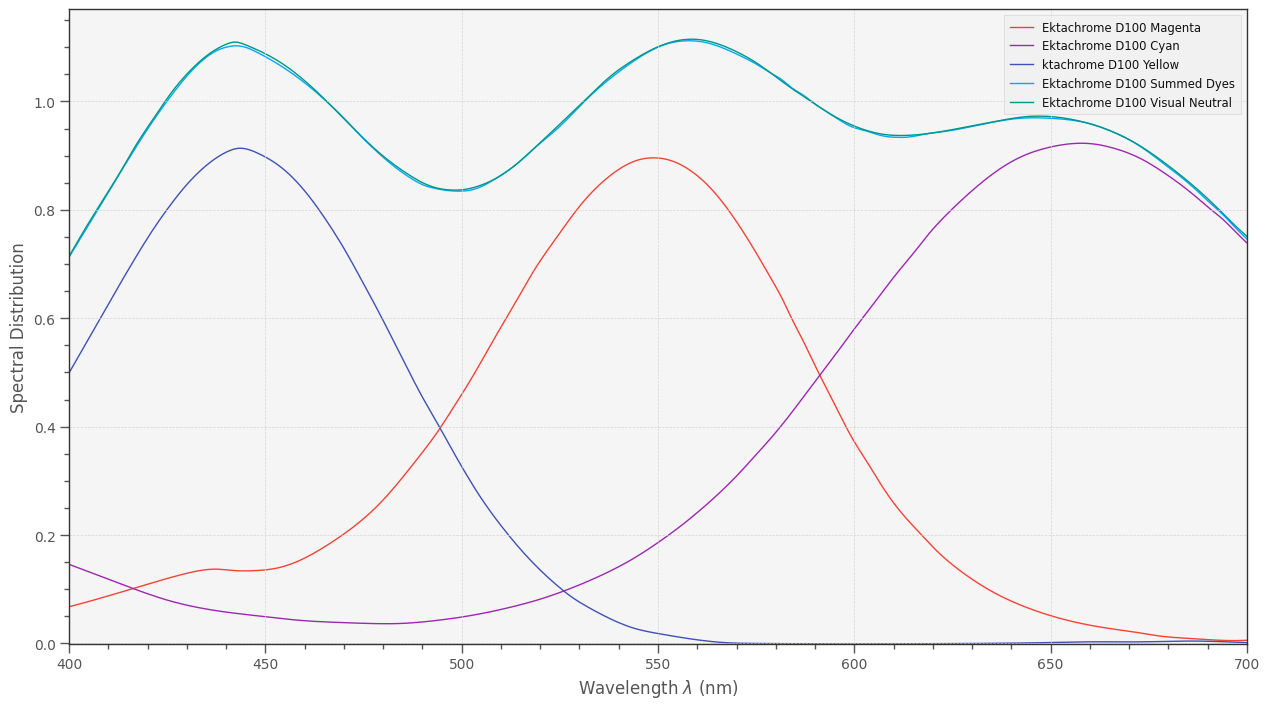
3. Created a third virtual color chart, this time using the spectral characteristics of Ektachrome 100 D (“Ekta”).
4. Created a virtual camera simulating capture of the color charts with a Raspberry Pi HQ sensor.
5. Computed the difference of what the camera recorded in comparision to the reference color chart under various different illumination setups.

With respect to point 4., that is, the virtual camera, I implemented basically two different functionalities of the camera:

1. Operating the camera via libcamera/picamera2. That means:

• Estimate the appropriate whitebalance from the illumination spectra. That is: adjusting the red and blue gains to the illumination. Could be done also manually, does not matter too much.
• Reading in the information from the scientific tuning file.
• Estimating a correlated color temperature (cct) from the given red and blue channel gains.
• Using that color temperature to calculate a CCM transformation matrix from the ones stored in the scientific tuning file.
• Using that CCM to compute the colors “seen” by the camera.

2. Alternatively, using an optimized CCM for computing the resultant colors, in effect bypassing libcamera (similar to raw captures). The optimized CCM was derived from either the virtual Kodakchrome 25 or the virtual Ektachrome 100D color chart:

• Taking an image of the color chart used for calibration under a defined illumination.
• Run an optimizing scheme trying to come up with a transformation matrix mapping as closely as possible the resulting colors onto the reference target. This is the most simple direct CCM approach possible; more advanced software includes the possibility of 1D or even 3D LUTs to be thrown into the processing path - I have not implemented these more advanced approaches.

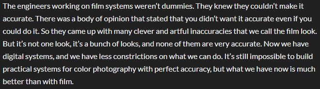
Here’s the simulation result using a blackbody radiator with 3200K (see the last plot of this post for the illumination spectra used here) with the various cameras implemented:

I use here the blackbody radiator with 3200K as illumination. This should be quite similar to the Tungsten lamp used when projecting S8-footage in the old days.

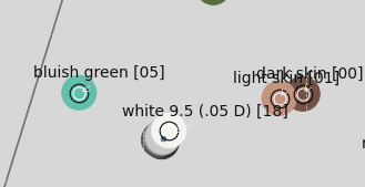
Some explanation on how to read this display is appropriate here. Overall, it shows how the patches of a virtual color chart would be recorded by our virtual camera. For each patch, the central area (“Inset”) shows how the reference color chart would be seen under D65 illumination. Around that center patch, the segments show the results of various simulation runs.

Specifically, this chart shows the appearance of the Kodachrome 25 based color chart illuminated with a 3200K blackbody radiator, for various different processing schemes:

• libcamera: the CCM is computed by libcamera/picamer2, as described above.
• Direct, Kodak Ref: the CCM used was optimized with the Kodachrome 25 color chart
• Direct, Ekta Ref: the CCM used was optimized with the color chart realized with Ektachrome 100D dyes.
• Direct, D65 Ref: the CCM was computed based on the color chart using print dyes, not film dyes.

Visually, it seems hard to notice any differences with respect to the different processing schemes. All simulated “cameras” performed quite well.

The data values listed besides each entry give a more quantitative information:

• ΔE mean - is the average color error of the set.
• ΔE std - is the standard deviation encountered.
• ΔE min - is the minimal error found.
• ΔE max - is the maximal error found.

For the min and max-entries, the patch found is indicated by the number in [..].

The best performance on a Kodachrome target is obtained with the direct method (calibrated CCM) using the Kodachrome color chart for calibration. Not too surprising, actually. Using instead the Ektachrome chart as calibration reference, we see a slightly larger ΔE = 0.89. An even larger one, ΔE = 1.23 results when using the color chart based on print dyes. So this set of simulations shows that the dyes used in the calibration chart used does matter. Remeber, the “Ref” is using print dyes, “Kodak” is using Kodachrome dyes and “Ekta” is using Ektachrome dyes. Ideally, one should use the dyes of the material which is planned to be scanned for calibration.

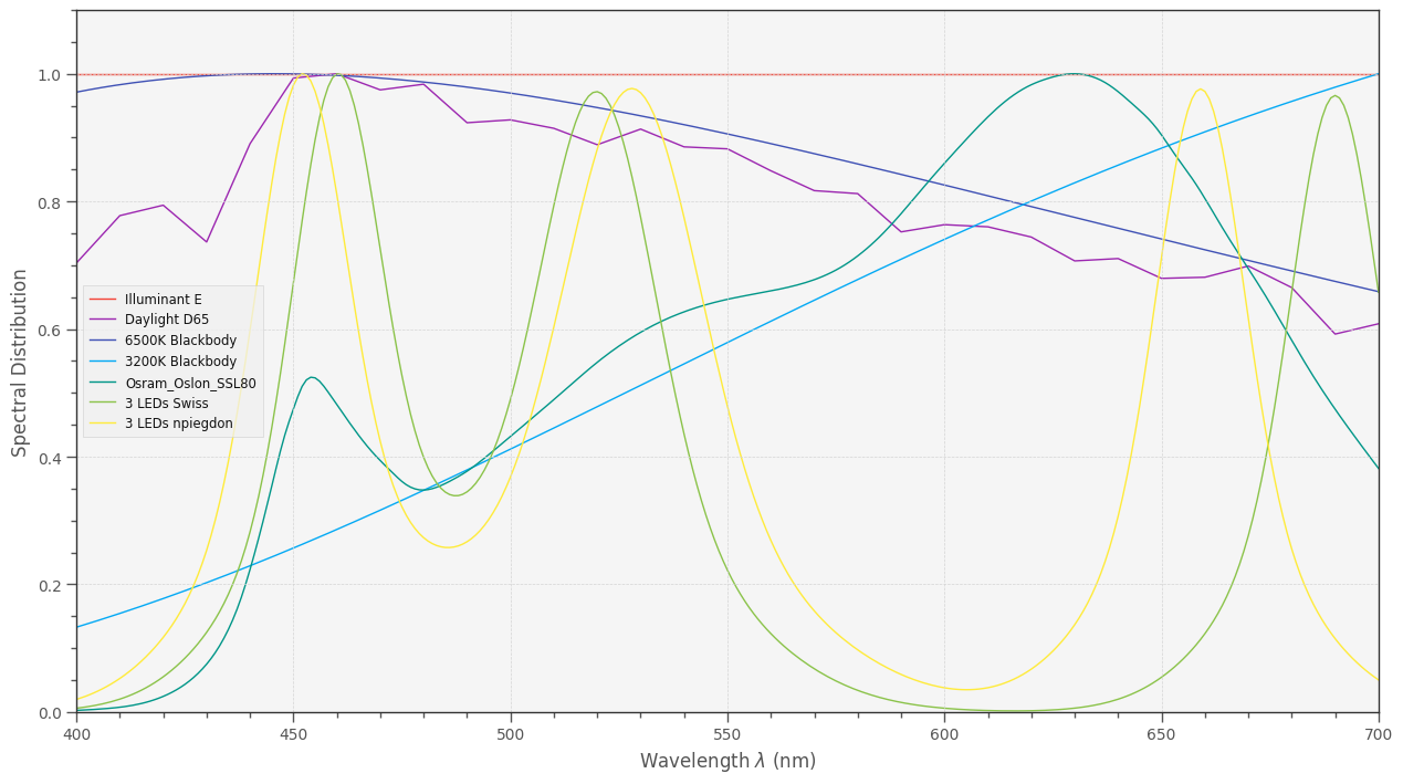
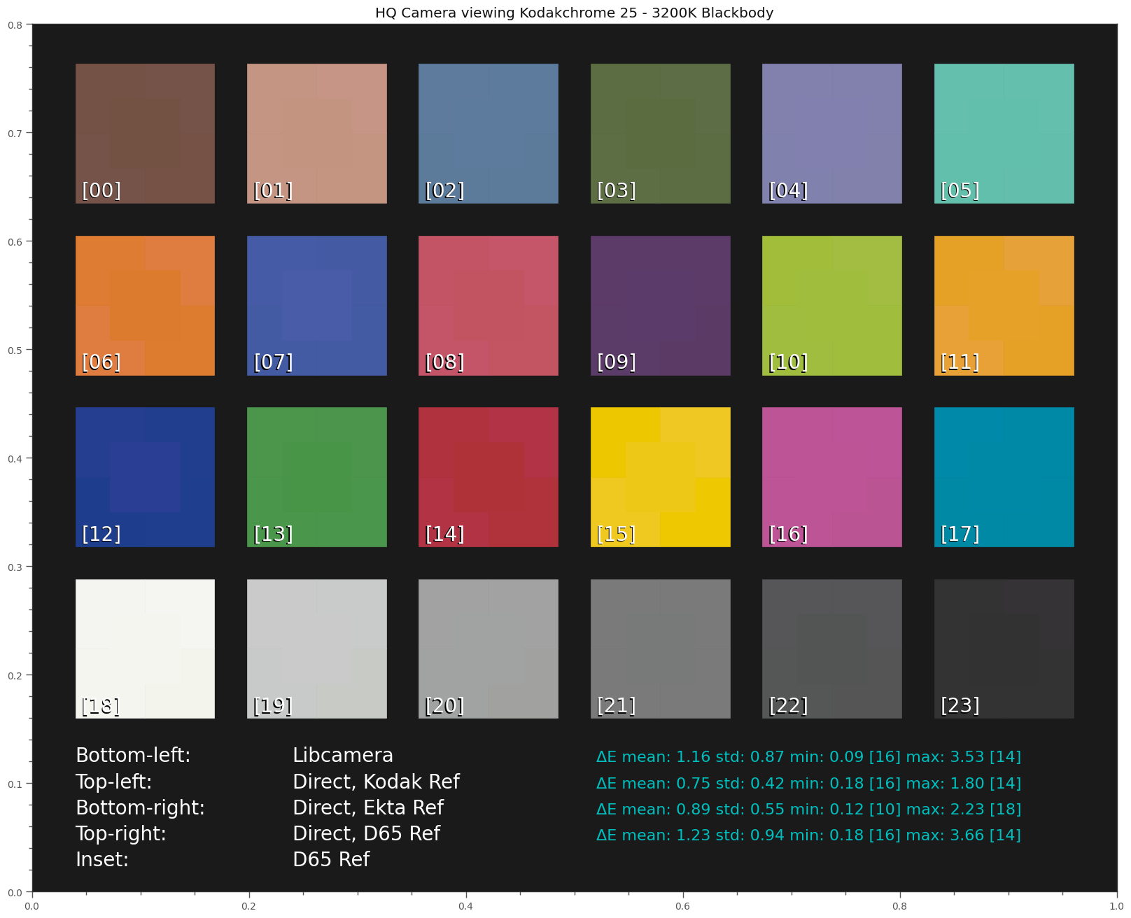
Ok, next. The following chart examines the influence of different illuminations under the standard libcamera/picamera2 processing, using the scientific tuning file. The various illuminations are used to estimate a correlated color temperature and this color temperature is in turn used to compute the CCM transformation matrix for the camera. Specifically, the following illumination have been tested:

3200K Blackbody:                   Estimated cct:  3200.0
SSL_80:                            Estimated cct:  3146.93236375
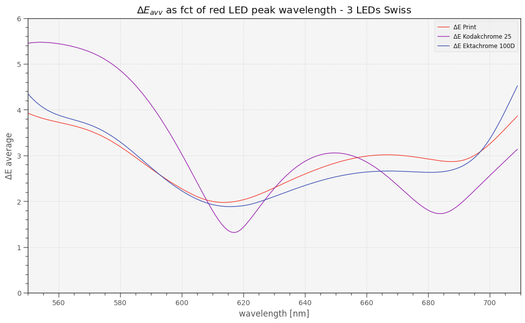
3 LED Swiss:                       Estimated cct:  7772.82512135
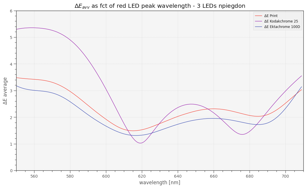
3 LED npiegdon:                    Estimated cct:  7403.21605312

One can already see that the estimated color temperatures of the three LED setups are way off. In fact, narrowband LED illumination does not really have a correlated color temperature (cct).

Anyway - let’s see the simulation results:

Yep, the results are as expected. Both 3 LED setups show quite noticable deviations in color appearance compared to the 3200K blackbody illumination. The main difference between “Swiss” and “npiegdon” is the position of the red LED - obviously, the placement of the narrowband LEDs within the spectrum has an influence upon the color fidelity. The later has only half of the color error than the Swiss one.

Note that the modern day bulb substitute, the “SSL_80” broadband LED, even yields better results than our reference illumination “3200K blackbody” - however, the difference is tiny. The overall simplicity of our simulation approach does not allow us to draw any conclusions from such small deviations.

Ok. So pairing narrowband LED illumination with standard libcamera/picamera2 processing is probably not such a good idea. Note that when working with .dng-files, your raw converter will use the CCM computed by libcamera by default - that is a result of the way picamera2 creates the .dng-file.

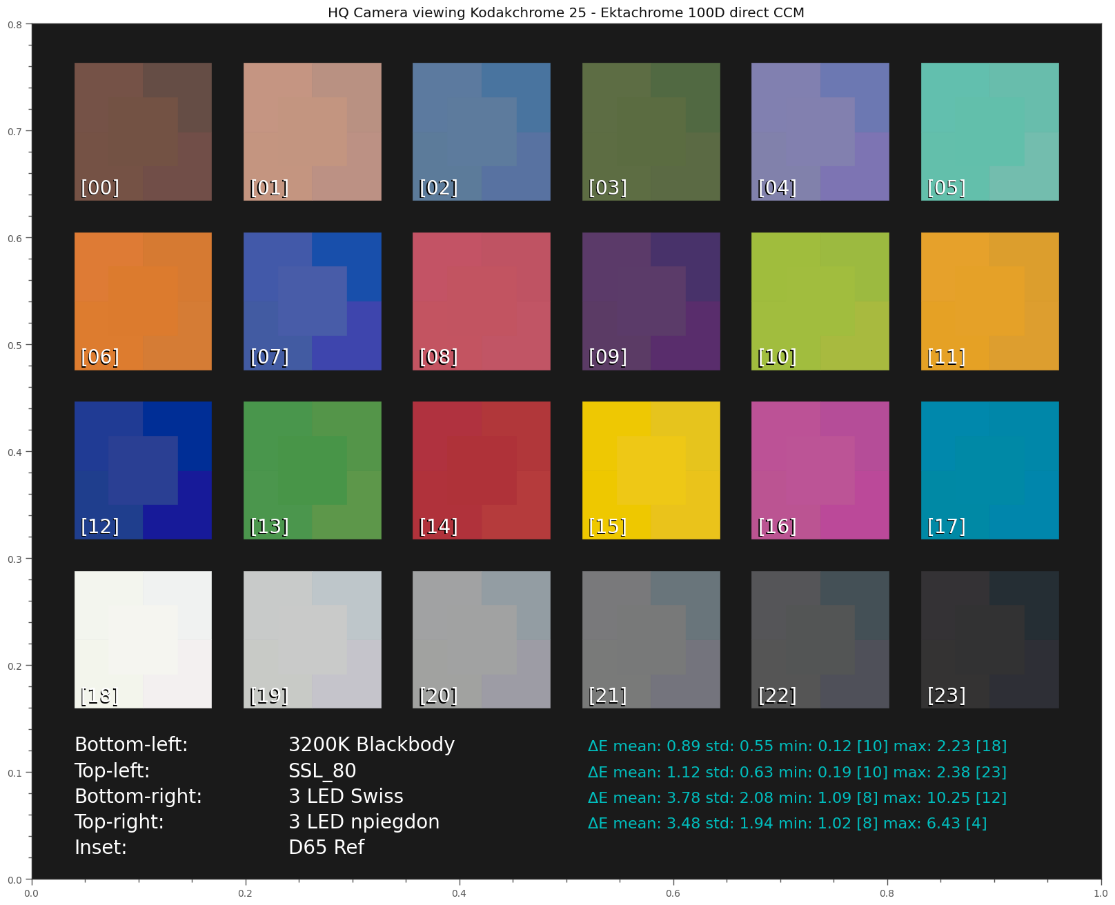
Well, we can do better if we compute an optimized CCM based on a previous calibration run.

Here are the results of calibrating with the film dye based Kodachrome 25 color chart

under various illuminations. All ΔE improved - as expected.

Note that a calibration using only a CCM is a rather simple approach - usually, there would be either 1D LUTs or even 3D LUTs thrown into the calibration recipe here. However, I neither do have software available for calculating LUTs, nor is a simple 24 patch color checker sufficient to guess the many values required for a LUT. So that’s all I can offer in terms of calibration-based CCMs.

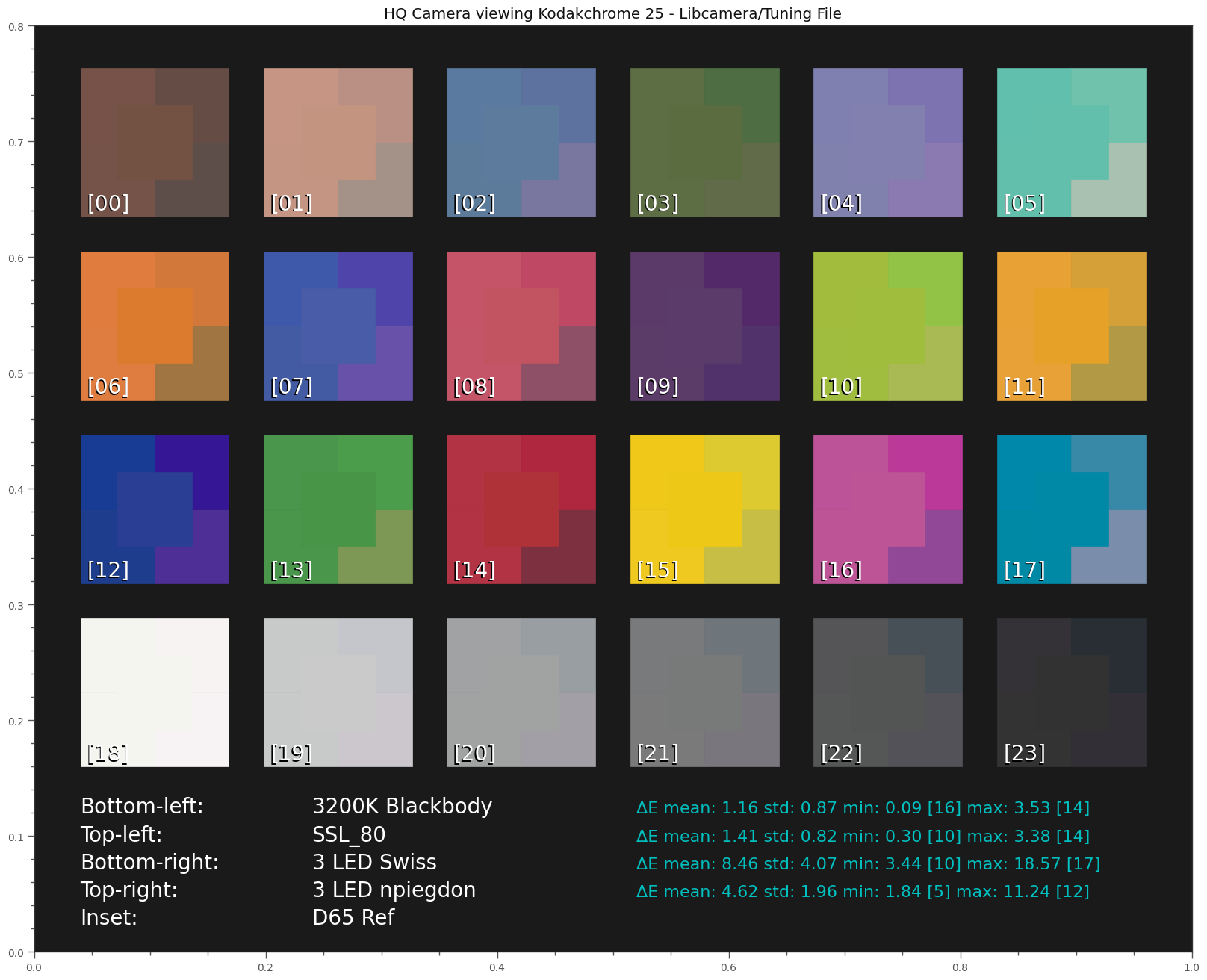
Ok, lastly, let’s check what happens if we do not base our calibration on a simulated Kodachrome 25 color chart (which uses the same dyes as the scan), but a simulated Ektachrome 100D (which uses different dyes).

Well, here’s the simulation result:

As expected, the ΔE get slightly worse. Since we are using the wrong color chart (“Ekta”) with dyes different from the media we actually scanning (“Kodak”), this is not really a surprise. But the drop in fidelity is not as big as I expected.

Summarizing what I have learned by this journey:

• The combination of a modern broadband whitelight LED with libcamera/picamera2 processing based on the scientifc tuning file should yield quite acceptable color fidelity.
• Using narrowband 3 LED based illumination with a calibration yields comparable results - even if the calibration target is not identical to the film stock scanned.
• The results of narrowband 3 LED illuminations seem to be extremely sensitive to the wavelengths of the LEDs used.

[npiegdon]

@cpixip

However, I neither do have software available for calculating LUTs, nor is a simple 24 patch color checker sufficient to guess the many values required for a LUT.

This part isn’t too tricky. You start with a chart layout from Argyll. See any .cht file in the argyll/ref folder. They’re just text and the format is straightforward. Wolf’s layout is in the folder (it8Wolf.cht). So are a few ISO 12641 layouts (along with lots of others). They’ve each got hundreds of reference patches along with the positioning info.

Write the kind of simulated image (under a given virtual light source) like you’ve been doing above, with all the patches in the right place. Then write the spectral data for each patch out to a sidecar text file (the same way all the other reference data is written by everyone else: Wolf’s, SilverFast’s, gwbcolourcard’s, etc.)

Now you can run this tool:

bin/scanin.exe myColorChart.tiff ref/it8Wolf.cht colorPatches.txt

That generates a .ti3 file, which is the main interchange format for the rest of Argyll’s tools. (On this silly flow chart it’s the horizontal pink line about halfway down that separates most of the “input” tools from most of the “output” tools.

With the colorPatches.ti3 file in hand, all you have to do to generate an ICC file with an embedded 3D LUT is:

bin/colprof.exe -v -nc -ua -qh -ax -O output.icc colorPatches

The options mean:
-nc: don’t include the .ti3 data in the .icm files
-ua: Absolute Colorimetric intent
-q[lmhu] is quality { low, medium, high, ultra }
-ax: XYZ cLUT

If High quality takes too long, Medium would probably be fine. (As we discussed a while back, Ultra takes very long and is almost certainly overfitting the data.)

Anyway, with the ICC file, the sky is the limit. There are tools available to convert those into the kind of .cube LUT that video editing packages prefer, but the ICC is already useful immediately with image editing tools like ImageMagick or Photoshop.

If you wanted to do the Delta E checking, they’ve got a tool for that which takes the 3D LUT into account:

bin/profcheck.exe colorPatches.ti3 output.icc

So for your purposes, is the only missing code the following?

• Read the XYZ values in the .cht file to tell you how to lay out the patches in your TIFF.
• Write the “reference” XYZ or spectral data to a CGATS-style file like all the other reference data out there.

[cpixip]

@npiegdon

This part isn’t too tricky.

Well, sort of. Your “silly flow chart” as well as the different data formats used by the software are not really inviting. Thanks for providing this great overview on how to perform scanner calibration with opensource software (Argyll) - that will help others who want to travel along this path.

I guess for me however this journey has come to an end, sort of - remember, I started my film scanning with various 3 LED setups, was not really convinced about the results and ended up with using a broad whitelight LED only. Lately, I reconsidered switching back to a 3 LED setup, but I had my suspicions that it might be a complicated endevour, maybe not worth the effort for me.

The reasons are varied; mainly I am guided by simplicity and resonable allocation of resources. That’s why I will stick to my current scanning paradigm, namely scanning under the control of libcamera/picamera2 raw image data and store them as .dng-files. Picamera2 includes in the .dng-file a scientific tuning file derived CCM which is used by default by most raw converters developing the raw. With my broadband whitelight LED, featuring a sufficiently high CRI, I end up with an approximate ΔE of close to 1.0, out of the box. That is absolutely good enough for me, especially when considering the following points:

• Conservation the film look - I have quite different S8-material, each with a specifc film look. “Film look” is of course a marketing phrase for “my film stock cannot reproduce the real colors of the scene”. In my final product, I want to have a compromise between the film look printed into the scene by the specific film stock used and the “true” colors of the scene.
• S8-film stock is not true to scene colors anyway - old S8 film stock had only two selectable color temperatures. “Tungsten” and “Daylight”. But: most of the time, the scene color was not even near those two standards. So, the colors recorded by the film stock were anyway slightly wrong, always. Here’s again an artistic decision hiding: In principle, you could use secondary color grading to match the colors of the foreground illuminated by fluorescent light to the colors of the background illuminated by bright daylight, for example. Or: you could keep it that way in your digital copy. Depending on the scene content, you might opt for either of these options.
• Modern viewing standards - people are nowadays used to color graded material. In fact, chances are you are going to end up in your workflow with some kind of color grading anyway. If so, all concerns about color fidelity will be thrown out of the window.

That is why I remarked previously that the discussion in this thread is more academic than practical. Also, the whole numerical experiments didn’t even touch the issue of faded film stock. That’s a totally different story where dynamic ranges of sensors and digital pathways need to be discussed. Since all my faded film stock is at most a few minutes of footage, that is of no concern for me at the moment. I am handling this material in the post.

Finishing here with one last “academic” result, by simulating a setup with the HQ camera and Swiss 3 LED illumination, assuming a CCM obtained by a previous calibration step. I shifted the peak position of the red LED over some range and obtained the following plot:

The actual value used in the Swiss setup is red = 690 nm. This value is actually close to a local minimum of the Kodachrome 25 curve. But not for the other color charts using different dyes. This shows the dependence of the optimal peak wavelengths of the LEDs with respect to the film material scanned - a complication which is impractical to circumvent. Also note that there is a global minimum, around 620 nm (however, the improvement will not be noticable). The position of the global optimum features a lot more overlap with the green LED at 520 nm, reducing blind spots in the spectrum introduced by the original 690 nm LED choice. However, most probably the channel separation is larger in the 690 nm position compared to the 620 nm position. So for faded material, this might be a better choice.

Doing the same game with your LED setup, where the blue LED’s peak is located at 452 nm (vs 460 nm of the Swiss setup) and the green LED’s peak at 528 nm (vs Swiss 520 nm) one obtains the following plot:

Note that the tiny shifts in the blue and red LED’s peaks reduced the overall error. Again, the differences will not be noticable - they are too tiny to matter.

Also note that I have used in this simulation not a monochrome camera as you are using in your setup. So the results are not really transferable. But it shows me that when using a 3 LED setup, the peak wavelengths of the LEDs used are actually critical. The optimal selection depends on the film stock scanned. That was in fact what I discovered when I was experimenting with such an setup in my inital scanner construction. Which brings things a little full circle for me.

(Disclaimer: I cannot rule out coding errors in creating any of the diagrams in this thread - these are the results of rather complex simulations. So take all results with a grain of salt.)

[Radoslav_Markov]

I always like when amateurs discuss matter they dont understand. A french book or color in 2013 clearly stated that gamut of CMY (subtractive capture/synthes) is different from gamut of RGB additive (capture synthes). I , at IBC 2017 stated the way to resolve the problem of scanning archive film material indifferent of the epoch, color system and ages in order to reproduce all colors.So, the problem is clear and the solution is clear you not need to spend your time with the things you barely understand.

[cpixip]

@Radoslav_Markov Hello and welcome to the forum! Great that you are joining the discussion.

@Radoslav_Markov

I , at IBC 2017 stated the way to resolve the problem of scanning archive film material indifferent of the epoch, color system and ages in order to reproduce all colors

Please enlighten us on your approach - this forum is very interested in new ideas for scanning old film stock. So again, join the discussion and share your knowledge with us!

[npiegdon]

I’ve been trying to find what he might have been talking about and bumped into this short column on page 63 of this magazine from the end of 2017:

Unfortunately, the URL doesn’t point to a live site and the Wayback Machine only has a few blank/404 entries for it.

@Radoslav_Markov, was this related to what you were trying to communicate?

[PM490]

I have seen much “stated” at IBC and NAB that is not so.
Care to share your research and scanning results? Perhaps a video of your presentations?

[friolator]

@cpixip

Please enlighten us on your approach - this forum is very interested in new ideas for scanning old film stock. So again, join the discussion and share your knowledge with us!

I would strongly recommend igoring Radoslav’s posts. He’s been trolling on the DIY film scanner facebook group for years. Basically only interested in telling everyone they’re an idiot.

[cpixip]

Here’s a short discussion about scanning negative film, specifically broadband vs narrowband illumination:

A Better Light Source For Scanning Color Negative Film

Might be interesting for the forum.