My 8mm/Super8 Scanner build (in progress, LED help)

[Manuel_Angel]

I agree with the opinion of @cpixip.

Although a procedure based on adjusting the lighting intensity should work in principle, it is not easy to put into practice.

Assuming that we could somehow adequately vary the intensity of the illumination, in my opinion we still have to deal with some undesired effect such as the change in the spectral composition of the light.

With the picamera2 library it is easy to change the exposure time, however, according to my tests and experiences, the change is not immediate.
In my software, prior to taking a capture, I run a loop where the desired exposure time is compared with the exposure time reported by the camera’s metadata. When both times coincide within a tolerance of 50 us, the loop is exited and the image is captured.

Specifically, I use this loop after the change in the exposure time and before capturing the image:

#This loop has the function of ensuring that the camera uses
# the new exposure time.

            numOfRetries = 0

            for i in range(config.numOfRetries):
                numOfRetries += 1
                metadataExposureTime = self.cam.captureMetadata().ExposureTime
                dif = abs(bracketExposure - metadataExposureTime)
                # info("Theoretical exposure time = " +
                #       str(bracketExposure) + " us\n" + " "*29 +
                #       "Camera real time = " +
                #       str(metadataExposureTime) + " us\n" + " "*29 +
                #       "Difference = " + str(dif) + " us")
                if  dif <= config.timeExpTolerance:
                    break

            # info("Number of retries = " + str(numOfRetries))

To my surprise, although the picamera2 library does not use the GPU, it is faster than the old picamera library.
With the RPi 4 a capture that with the old library took an average time of 4 s, in the same conditions with the new library the time has been reduced to 2.6 s.

[PM490]

I agree with the suggestions by @cpixip and @Manuel_Angel to use the camera exposure change approach. I explored the option for changing the light intensity, and the implementation is not as simple as the option to change camera exposure.

@Manuel_Angel

Assuming that we could somehow adequately vary the intensity of the illumination, in my opinion we still have to deal with some undesired effect such as the change in the spectral composition of the light.

@Manuel_Angel, from experimenting with White LEDs, it is possible to control the intensity (example implementation in this post). The results of the experiment do not show a significant change in the white balance (light spectra) at the range appropriate to the camera used, note this video of the implementation with a DSLR D3200.

The best of both worlds may be a tap approach to increase light intensity for capturing the ultra-dark portions of the scene. That can be done by turning on/off an extra LED set without the complications of intensity control.

[d_fens]

thanks for all the feedback,

one thing that crossed my mind why changing the lighting might be an advantage:

for the very dark areas of a (underexposed) film the light passing through without burning out highlights might not be bright enough to recover dark details, no matter how long the exposure time?

do you think this is a valid point or event important?

[cpixip]

– adding here some additional information about delays and cyclic capture. When you request a certain exposure time, libcamera/picamera2 will need quite some time to give you that exposure time back. Here’s the output of an experiment I did about a year ago (so this is an old version of picamera2):

 Index - requested : obtained : delta
  0 -     2047 :     2032 :   0.031 sec
  1 -     2047 :     2032 :   0.034 sec
  2 -     2047 :     2032 :   0.034 sec
  3 -     2047 :     2032 :   0.044 sec
  4 -     2047 :     2032 :   0.031 sec
  5 -     2047 :     2032 :   0.034 sec
  6 -     2047 :     2032 :   0.034 sec
  7 -     2047 :     2032 :   0.044 sec
  8 -     2047 :     2032 :   0.031 sec
  9 -     2047 :     2032 :   0.034 sec
 10 -      977 :     2032 :   0.031 sec
 11 -     1953 :     2032 :   0.021 sec
 12 -     3906 :     2032 :   0.035 sec
 13 -     7813 :     2032 :   0.032 sec
 14 -    15625 :     2032 :   0.033 sec
 15 -      977 :     2032 :   0.034 sec
 16 -     1953 :     2032 :   0.033 sec
 17 -     3906 :     2032 :   0.032 sec
 18 -     7813 :     2032 :   0.033 sec
 19 -    15625 :     2032 :   0.034 sec
 20 -      977 :     2032 :   0.037 sec
 21 -     1953 :      970 :   0.029 sec
 22 -     3906 :     1941 :   0.038 sec
 23 -     7813 :     3897 :   0.028 sec
 24 -    15625 :     7810 :   0.036 sec
 25 -     2047 :    15621 :   0.033 sec
 26 -     2047 :      970 :   0.032 sec
 27 -     2047 :     1941 :   0.037 sec
 28 -     2047 :     3897 :   0.030 sec
 29 -     2047 :     7810 :   0.032 sec
 30 -     2047 :    15621 :   0.034 sec
 31 -     2047 :      970 :   0.033 sec
 32 -     2047 :     1941 :   0.036 sec
 33 -     2047 :     3897 :   0.031 sec
 34 -     2047 :     7810 :   0.034 sec
 35 -     2047 :    15621 :   0.035 sec
 36 -     2047 :     2032 :   0.031 sec
 37 -     2047 :     2032 :   0.034 sec
 38 -     2047 :     2032 :   0.034 sec
 39 -     2047 :     2032 :   0.044 sec

For frames 0 to 10, the exposure time was fixed at 2047 - but I got only a real exposure time of 2032, the rest “taken care of” by a digital gain larger than 1.0.

At time 10 I request a different exposure time of 977. The first frame with that exposure time arrived only at time 21. That’s the time the request needed to travel down the libcamera pipeline to the camera and back again to picamera’s output routine. Eleven frames is more than a second in the highest resolution mode! Again, I requested 977 and got 970 - close, but not a perfect match.

After time step 10 I cycle through all the exposure values, that is [977,1953,3906,7813] for a few cylces. As you can see, the camera follows that cycle frame by frame. Once I switch back to my base exposure 2047 at time point 25, the camera continues to cycle until time 36 where it delivers again the requested exposure time.

So - in order to get the data of a full exposure stack, in cycle mode you need to wait only for four consecutive frames at most. Provided, you cycle constantly through all exposures. Given, you have no idea which of the four exposure will be the first to show up in the pipeline, but you know that the following three frames will be the other missing exposures. That’s the neat trick of cycling constantly through all required exposure. I got this trick from David Plowman, the developer of picamera2.

Of course, you need to program some logic which will save the incoming data into the appropriate slots of your HDR-stack, and you will need some additional logic to trigger frame advance and wait a little time that all the mechanical vibration have been settled.

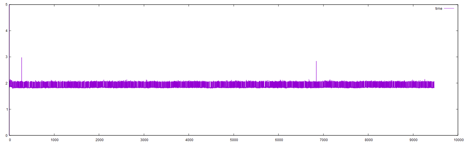
As my scanner is mechanically not very stable (it’s all plastic), my waiting time (time between “trigger of frame advance” until “store next frame in HDR-stack”) is 1 sec; running the HQ sensor at it’s highest resolution gives me a standard frame rate of 10 fps. Nevertheless, capturing a single HDR-stack of a frame takes me on the average between 1.85 and 2.14 sec. Here’s a log-file of such a capture (capture time vs. frame number):

Note that these times include my 1 sec mechanical delay. So the capture would be faster if your mechanical design does not need a long movement delay. Again, this is the result when using the HQ sensor at full resolution setting, i.e., with 10 fps.

Occationally there are spikes where the capture takes noticeably longer, about 3 sec (two in the above plot). Might be related to some syncing issue, but I do not know the real reason. As it does not happen very often, I did not bother to investigate further.

[cpixip]

@d_fens

for the very dark areas of a (underexposed) film the light passing through without burning out highlights might not be bright enough to recover dark details, no matter how long the exposure time?

do you think this is a valid point or event important?

Short answer: no

The range of exposure times is much larger than the range of illumination settings you might have available for your illumination. An extra boost of doubling the intensity of a LED requires approximately to double the current flowing through the LED - but all LEDs have some current limit…

If you really want to have a strong shadow-push, you would need to work with a quite dim LED setting for normal scenes - this gives you potentially more noise from other sources (for example stray light from your environment will be more noticeable).

On the other hand, doubling the exposure is basically for free - you just need to scan a little bit slower.

Also, from my experience, a HDR-stack with 4 to 5 exposures is really sufficient for most film material. The important point is to fix the fastest (darkest) exposure in such a way that no highlights are blown out. That is, the brightest image areas should have values around 240 in an 8bit/channel image. I call this image “highlight image”.

The next image in the HDR-stack should have double this exposure time. You will discover that this image is generally quite a good scan of its own. That’s the reason I call this “prime image”. Doubling again exposure time for the first shadow image (“shadow 1 image”) and again for the second shadow image (“shadow 2 image”) and you should be done for all practical purposes. The shadow details you are capturing with this approach will display quite a noticeble film grain and under usual circumstances will end up anyway as rather dark areas in your final grade. That’s why I switched at some point from five exposures to only four - its sufficient for all practical purposes.

A note on this: I do have Agfachrome MovieChrome film stock which cannot be captured in full glory even by the five exposure approach. In very blue areas (sky), the red channel absorbs an incredible amount of light, staying pitch dark even in the brightest exposures. So far, I have not found a way to capture this faithfully - however, it plays no role in the exposure fused result I am currently working with. It is noticeble in a real HDR - but that issue is reserved for future endeavors.

[PM490]

@cpixip

On the other hand, doubling the exposure is basically for free - you just need to scan a little bit slower.

What about noise differences with long and short exposures?

[cpixip]

@PM490

What about noise differences with long and short exposures?

Good question! Generally, in a digital camera the noise is mainly connected on how the analog amplifiers are set. That is in picamera speak the analog gain. Digital gain has a similar effect and in addition reduces somewhat the number of available intensity values.

Doubling the exposure time should not lead to increased noise per se. Just another range of illumination intensities will be mapped to the output range. For scanning operations, one should always use the lowest gains possible.

From another point of view, small format film stock is incredible noisy in dark areas - if you double exposure time, the film grain becomes quit visible and annoying in dark areas. Luckily, those areas end up in the final edit also in the rather dark regime…

[PM490]

@cpixip

Generally, in a digital camera the noise is mainly connected on how the analog amplifiers are set. That is in picamera speak the analog gain. Digital gain has a similar effect and in addition reduces somewhat the number of available intensity values.

Agree.

@cpixip

For scanning operations, one should always use the lowest gains possible.

Agree.

@cpixip

Doubling the exposure time should not lead to increased noise per se.

Provided a constant gain, I think is the opposite. The sensor has inherent noise, and if larger exposure provides a larger Signal the result should be an improved signal/noise at larger exposures, when illuminant intensity remains constant.

This article explains the particulars, some of it is beyond my depth of knowledge. This astro-photography review seems to reach the same conclusion.

@cpixip

If you really want to have a strong shadow-push, you would need to work with a quite dim LED setting for normal scenes - this gives you potentially more noise from other sources (for example stray light from your environment will be more noticeable)

The above hypothesis does not consider ambient light noise.

If my understanding is correct, it would indicate that there may be advantages on decreasing the light intensity for lighter image exposure.

Another interesting conclusion is that in general, stop motion with larger exposures (and less light), would give a better Signal to Noise than continuous motion which requires much shorter exposures (and more light).

[cpixip]

@PM490

@cpixip

Doubling the exposure time should not lead to increased noise per se.

Provided a constant gain, I think is the opposite. The sensor has inherent noise, and if larger exposure provides a larger Signal the result should be an improved signal/noise at larger exposures, when illuminant intensity remains constant.

This article explains the particulars, s

Well, the article supports my statement. Doubling the exposure leads to an increase of the signal-to-noise-ratio, that is, to better noise performance.

Generally, camera noise is a complicated beast and depends on the specific application setting. Your references deal with low-light situations, something we should not have in a scanning application.

Your second reference falls into the trap of the many different sources of noise. In order to get his comparision shots, he pushes very dark exposures by one or even two stops. This is equivalent to changing digital gain on your camera from 1.0 to 2.0 or even 4.0. In his experiment, he reduces dynamic range during image capture, but enlarges it again in postproduction. This is not a valid approach for analyzing camera performance.

In any case, the use case “astrophotography” is quite different from a scanning application. In a scanning application, you will want to work with as much light you can. Your camera will perform better and light coming from other sources than your film frame will be less noticeable in the scan result. The later point is especially import if your scanner has an open design (as my scanner has. Usally working in a darkroom because of this).

[PM490]

@PM490

@cpixip

Doubling the exposure time should not lead to increased noise per se.

Provided a constant gain, I think is the opposite.

You are right, I misread as halving the exposure… my bad.

@cpixip

Your second reference falls into the trap of the many different sources of noise. In order to get his comparision shots, he pushes very dark exposures by one or even two stops. This is equivalent to changing digital gain on your camera from 1.0 to 2.0 or even 4.0. In his experiment, he reduces dynamic range during image capture, but enlarges it again in postproduction. This is not a valid approach for analyzing camera performance.

Agree, the gain change is done in post, rather than at the sensor processing chain, the effect is the same.

[npiegdon]

@cpixip

That’s the neat trick of cycling constantly through all required exposure. I got this trick from David Plowman, the developer of picamera2.

That is a neat trick!

@cpixip

@PM490

This article explains the particulars…

[…] Generally, camera noise is a complicated beast and depends on the specific application setting. Your references deal with low-light situations, something we should not have in a scanning application.

What are your opinions about the exposure-averaging parts of the article? Assuming a high-illumination, (relatively) short exposure environment like the one we’re interested in, it seems like our use case would be closer to the “Read Noise Limited” side of all those graphs. (I got lucky and my Gen3 Pregius sensor is actually listed in the graphs, so I don’t have to even guess about it.)

I didn’t have the mathematical foundation they built up in the article, but my own testing has shown that averaging ten or more exposures reduces sensor noise dramatically. I hadn’t gotten as far as quantifying it yet, but the noise in a single-exposure image vs. an average of many exposures is readily apparent just by looking at them side-by-side.

That’s 10x (nearest-neighbor) zoom of neutral gray captures. The difference between averaging 10 or 20 exposures is imperceptible, at least to my eye. When the time came, I was going to try and find the sweet spot by graphing the standard deviation across a wide range of exposure count. I’m guessing the best tradeoff between total capture time vs. sensor noise will be in the single digits for number of exposures.

In any event, for non-continuous scanners, this seems like one of the easiest wins for squeezing out an extra dB or two of SNR (assuming a vibration-free environment).

[cpixip]

@npiegdon

What are your opinions about the exposure-averaging parts of the article?

Well, an interesting topic. Upfront, if we are talking about scanning Super-8 color reversal film, one should be aware that the film grain of the source will exceed the sensor noise of any decent camera by far. So the discussion is more on the academic than the practical side.

Anyway. Averaging multiple sensor readings is a simple and trusted way to get a higher signal-to-noise reading, trading in longer aquisition time for less noisy signals. If you know the type of noise (which you usually don’t do) you can even devise better schemes for noise reduction than just simple averaging.

So while averaging is a way to increase signal-to-noise ratios, it also increases, as you pointed out, the overall dynamical range of your data. However, assuming that the noise we are talking about is coming from independently distributed gaussian sources (the ideal case; of course, it is not), the improvement scales only with the square root of the numbers of captures.

Probably a better approach for increasing the dynamic range of your data is to use different exposure times for each of your captures. That is: create a HDR-stack ( a stack of LDRs (low dynamic range images) with varying exposure time).

Now, a HDR-stack needs to be converted into a single frame for display. There are basically two options here. One is what I call “real HDR”, which is a floating point image containing the radiance values for the frame.

This “real HDR” is normally a rather boring (flat/un-viewable) image which needs to be tone-mapped in a second step. This gives you a LDR image which you can view nicely with current display technologies as the output (That is the Debevec-algorithm with some tone-mapping of your choice.).

The other technique is exposure fusion (“Mertens”), which goes directly from the HDR-stack to a LDR output frame, without intermediate real HDR-image. As this algorithm mimics partially the image processing of your visual system, the results are usually quite viewable.

Whatever option you choose, hidden within both algorithms are averaging steps which will reduce the sensor noise - how much depends on the specific parameters you choose. So in a way, capturing a HDR-stack and converting that stack into a single LDR frame for your audience is probably preferable compared to capturing several images with equal exposure and averaging.

[npiegdon]

Following up on this, I ran the experiment where I measured the standard deviation of (16-bit, monochrome) image pixels after each successive identical exposure was averaged into the final result (all the way up to combining 127 exposures).

These were exposures of an S8 frame in the ReelSlow8’s (upcoming) film transport. It wasn’t under any sort of tension control (just the friction of unpowered stepper motors on either end as they haven’t been wired up yet), so I think all of the behavior seen after the first half-dozen exposures of each trial can be explained by the film loosening ever so slightly over the course of the minute or two it took to run all five trials. (If you look carefully, the drooping of each plot is weaker for each successive trial. And looking at the raw data before it was centered on each median, the trial plots don’t overlap and are monotonically decreasing.)

In any event, it’s pretty clear that you reach just about the best you’re going to get sensor-noise-wise after only a very few exposures. Three if you’re in a hurry. Or five if you want to be sure.

@cpixip

Whatever option you choose, hidden within both algorithms are averaging steps which will reduce the sensor noise - how much depends on the specific parameters you choose. So in a way, capturing a HDR-stack and converting that stack into a single LDR frame for your audience is probably preferable compared to capturing several images with equal exposure and averaging.

All of that was great advice, thank you. And now that I’ve seen that the number of exposures it takes to get the sensor noise out is essentially the same as it takes to build a reasonable HDR/Mertens stack for this type of subject, I agree that it seems like we’re able to solve both problems simultaneously. Nice!

[cpixip]

@npiegdon

Following up on this, I ran the experiment where I measured the standard deviation of (16-bit, monochrome) image pixels after each successive identical exposure was averaged into the final result (all the way up to combining 127 exposures).

These were exposures of an S8 frame in the ReelSlow8’s (upcoming) film transport. It wasn’t under any sort of tension control (just the friction of unpowered stepper motors on either end as they haven’t been wired up yet), so I think all of the behavior seen after the first half-dozen exposures of each trial can be explained by the film loosening ever so slightly over the course of the minute or two it took to run all five trials.

@npiegdon: very interesting experiment! I think one sees clearly that you get the most improvement through the first few frames. Two things: first, the standard deviation should not become negative, so it is a little bit unclear what is actually plotted in your graph. Second: even tiny movement of your frame will spoil the averaging procedure, because the texture the camera is grabbing changes. I do not know at what resolution you were capturing, but just calculate the size of a single pixel on your frame - you will be astonished how small that turns out. If your film moves only a fraction of this size, you are going to average over different image areas - which will twist your results at least a little bit. However, as you are interested solely in your camera’s noise (and how that behaves with averaging over several captures), you might as well skip the S8 Ektachrome frame and choose a main exposure of the empty gate which gives you about an average brightness value.

I also must confess that I simplied my argument about averaging in HDR work a little bit. Let’s look into this in more detail! The averaging you have in exposure fusion (“Mertens”) or a real HDR (“Debevec”) somewhat different from the summation you did above. This averaging uses a weight function. Here’s an example from an old prg of mine implementing Debevec:

The gray curve is actually the weight curve used in computing the HDR - it’s a gaussian. It does not use too dark (noisy) or too bright image areas (too burned out). Your averaging above would correspond in this graph to a constant straight line at the peak level of the gaussian. There are quite a few weight curves you can invent, resulting in different HDR reconstructions; one which would come close to your averaging would be a curve similar to the one depicted below

(Just for the curious: this is a multi-purpose display. The red, green and blue lines close to each other represent the calculated gain-curves of the camera. The gray curve represents the currently active weight function. The dotted line data points are the intensities of the HDR-stack images for a selected pixel, remapped to the common HDR image space. Ideally, they should all be on a straight horizontal line - there are clearly some deviations. Nevertheless, the red, green and blue bars on the right side of the display indicate the weighted sum of all pixels - in this case this was a gray pixel, so the RGB-values are quite similar. Finally, the red bar on x-axis indicates the current smoothing parameter for the estimation of the gain-curves. This parameter can be varied to optimize the gain curve calculation. By the way, another trick for this task is to use two different weight functions for gain curve estimation and HDR reconstruction. That’s the reason why I implemented quite a few different weight functions.)

Back to the topic: the exposure fusion algorithm “Mertens” uses also a gaussian quite similar to the one in the above first plot. At least in my implementation - which is slightly different from the one available in the opencv-library.

So, in summary, I did simplify my argument a little bit. Noise reduction with the “Debevec” or “Mertens” algorithm depends on a lot of things, most notably on the number of LDRs included in a single HDR-stack and the spacing of the exposures (half an f-stop, one f-stop, etc.), as well as the parameters of the weight functions used. Overall, if you are scanning S8 material, the film’s grain will outnumber by far the camera’s noise.

[npiegdon]

@cpixip

… the standard deviation should not become negative…

Each trial was centered on its mean so the lines could be compared more easily. (I mentioned it in the graph title, but in the following paragraph I said “median”, which is a mix-up of the two terms that I commit on a daily basis.)

If you don’t center them on the mean, you can still draw the same conclusions, but it’s harder to see from the graph alone:

That’s the plot of the raw standard deviation data. Here it’s much easier to see the “slowly losing tension on the S8 frame” effect I mentioned. I stopped for a minute or two after the first trial to make sense of what I was seeing, which I’m guessing is why there is such a large gap between the “Trial 1” and other plots.

It would have been better to wait until I have control of the tension or, like you suggested, just run the experiment on an empty gate. So I did and here are the results.

With an empty gate you get exactly the curve shape you’d expect for frame averaging. The perfectly aligned plots on the “centered on the mean” left-hand side are nice. Maybe averaging around eight frames is better in the conservative case?

The slight vertical shift in the raw data for the last two trials can probably be explained away by temperature effects on LED or camera. I stopped gathering data for a couple minutes between trials 3 and 4 while the blue LED was running continuously on my light board’s “high” setting. So presumably something was getting warmer, which offset the measurements for those last two trials. The camera body does eventually become quite warm, so this is a good reminder that these machines may require a warm-up period before each session to get the most consistent results. (It’s less important for the LEDs on an intermittent motion machine, where their duty cycle will be in the single digit percentages. Running them continuously in this case was out of the ordinary.)

@cpixip

Overall, if you are scanning S8 material, the film’s grain will outnumber by far the camera’s noise.

This is an interesting point. I suppose I don’t know how different types/shapes of noise compose. Handwaving nearly all of the math away, and just looking at the max, raw gray frame std.dev (around 350) vs. where it ended up after averaging many exposures (around 210), isn’t that effectively the same as gaining almost log2(350/210) = ~0.7 bits of signal? Even in the presence of S8 film grain, would that not still be true? Or is the strength of the S8 noise so overwhelming that this sensor noise is already down in the LSBs that are going to be thrown away during later processing steps like temporal denoising?

[PM490]

@cpixip

Overall, if you are scanning S8 material, the film’s grain will outnumber by far the camera’s noise.

This is true. However, I think the spatial nature of the sensor noise vs the 8mm grain is quite different. Moreover, when using a color sensor, there would be a noticeable color noise.
I would certainly agree that there is a trade-off where additional noise reduction for sensor noise may not be noticeable due to the spatially-larger film grain.

I am particularly bothered by the color noise of virtually every sensor, which significantly adds to the film not so colorful and larger noise.

[robinojones]

@PM490

I am particularly bothered by the color noise of virtually every sensor, which significantly adds to the film not so colorful and larger noise.

Chroma noise reduction using neat video really helps.I need to investigate if it’s possible in openCV. I would really love to add that in my post processing chain. Every sensor have this, neat video is the only plugin I know that doesn’t remove details when doing chroma noise reduction. Resolve DNR is bad in my experience.

[PM490]

@robinojones

Chroma noise reduction using neat video really helps

That’s what I used. The Nikon D3200 DSLR used in the first scanner is particularly bad, and Neat Video really did a great job.

[cpixip]

@npiegdon

@cpixip

Overall, if you are scanning S8 material, the film’s grain will outnumber by far the camera’s noise.

This is an interesting point. I suppose I don’t know how different types/shapes of noise compose. Handwaving nearly all of the math away, and just looking at the max, raw gray frame std.dev (around 350) vs. where it ended up after averaging many exposures (around 210), isn’t that effectively the same as gaining almost log2(350/210) = ~0.7 bits of signal? Even in the presence of S8 film grain, would that not still be true? Or is the strength of the S8 noise so overwhelming that this sensor noise is already down in the LSBs that are going to be thrown away during later processing steps like temporal denoising?

Well, yes, you can get another bit of camera depth by averaging over multiple exposures. You could alternatively combine a few raw exposures with different exposure times. Such a combination would practically be a HDR-computation with a simplified gain curve (it should be linear by default with most raw files). Combining several differently exposed raw images should be more effective in terms of improved bit depth, a little less effective on camera noise, as compare to averaging just a single exposure. And, of course, you could mix both approaches, that is, use for every exposure value a multitude of captures. That’s all possible. Question: is that worth the effort? Have a look at the following Kodachrome scan:

I can assure you that the sky visible in the background was a uniform gray background. A similar statement can be made for the hull of the airplane. So these image areas should show - ideally - just a constant color value. The structures you are seeing in these areas instead are film grain.

Frankly, I don’t think that the camera’s noise level plays any (noticeable) role here. Given, this Kodachrome film stock was treated badly - developed more than a year after initial exposure, under non-optimal storage conditions. I do have better developed Kodachrome stock with less grain. But I do also have other brands of film stock which feature even more grain than this Kodachrome example by default.

So - do I care about camera noise? As my primary target is grainy S8-material, not really. Do I care about the dynamic range of the capture? Certainly, as S8-material requires at least 12 bit of dynamic range.

[npiegdon]

@cpixip

Frankly, I don’t think that the camera’s noise level plays any (noticeable) role here.

I agree that image does appear reasonably free of sensor noise, or at least the JPEG artifacts are hiding anything that might have still been present.

What I mostly had in mind was the kind of egregious color noise that @PM490 was describing with the single-pixel rainbow speckles. In dark areas it can get pretty distracting. Although, I suppose that is exactly what the additional, longer HDR exposures are intended to fix.

@cpixip

And, of course, you could mix both approaches, that is, use for every exposure value a multitude of captures. […] is that worth the effort?

Once I get to the exposure fusion step, I was hoping to test both together in the way you described. My particular camera is streaming full-res, raw images at ~40 fps, so averaging several extra images together can be done in under 100ms. Doing that at each exposure value doesn’t seem like that bad of a time hit. (Especially when they’re “free” exposures that don’t need to wait for motor settling time or other changes in the system.)

That said, if there isn’t any perceptible difference, that is time that could be better spent making the rest of the process faster. I’ll try to quantify it when the time comes and–as always–report my results here. Thanks again for your input.