My telecine machine

Thanks Rolf, that was an impresive post. Certainly more information that I am able to digest in one go.
First I have to go through the links you provide, then I can see a couple of items to do in the short term (capture mode my camera is really using, using video capture instead of still), and some others for later on (client-server setup to handle exposure fusion).

There’s only one thing that confused me, your mention that ‘in actual capture mode, the requirements are even lower, as not every image captured is streamed’. If the exposure fusion is done in an external system, you have to stream all captured frames to it, right?

1 Like

Well, the camera needs several frames before any requested exposure time is actually realized. These frames are all dumped by the server, but never transmitted to the client.

Thanks Rolf.
Yes, that’s what Manuel told me, and I already did in my frustrated attempt at implementing exposure fusion directly on the Raspberry.

Hi Juan,

As a client-server example in Python you can also look at my YART project.
It’s similar to Manuel’s project but special attention is given to the object-oriented aspect, multithreading and network communication.
My scans are finished so I don’t think I’ll port this project to Bullseye/Picamera2 but it can be used as a starting point.

On the previous posts I can make the following remarks from my experience:

  • AWB auto white balance is not really recommended and can lead to strange results. It is better to set the RED and BLUE gains on a representative image and keep them afterwards. Color adjustments can be made in post-processing
  • The question of automatic exposure is controversial. In my opinion one has to distinguish between a professional film whose exposure has been controlled and which should be kept and an amateur film in which there may be clearly under or over exposed scenes, in which case automatic exposure may be useful.
  • As explained by Manuel and Rolf you have to ignore two or three frames after an exposure change and about eight for the calculation of the automatic exposure.
  • For HDR I chose to capture only 3 frames but distributed around the one in automatic exposure, this should be about equivalent to the 5 or 6 frames without automatic exposure

For the performances, it should be noted that the PI is severely limited by its hardware.
I made my captures in 1540x1080 (super8 ratio) it is also my post processing and encoding resolution without any crop (the lens is adjusted to have exactly the image on the sensor). The resolution 2028*1520 is still acceptable but the maximum resolution 4056x3040 is totally out of reach, it’s still a shame.

I did some inconclusive tests with Picamera2/libcamera, no performance gain, quite the opposite.
The gain of a 64 bits OS must be limited
On the other hand, the PI4 is a clear progress for the ES, the USB bus is faster and especially the controller is independent of the USB bus and really 1GB

Finally a remark about multitasking in Python, multithreading is adequate for IO-bound tasks (USB, network, camera) but not for CPU-bound tasks because there is no simultaneous execution of Python code. For example in my yart application there is the main thread a camera capture thread and a network sending thread.
So in your case yes you need a write thread but I don’t think that three brings anything.
For a CPU intensive application merge HDR, jpeg encoding, … you should do multiprocessing to take advantage of the quad core

2 Likes

Hi Dominique,

Thanks for your interesting remarks.

At this point I have learned a few things I’ll apply for my next scans, however I’ll take it easy since a couple of days ago I scanned my last remaining reel and for now I’m quite happy about the quality, since it is definitively an improvement over what my brother did 20 years ago filming the projections on the wall.

For the second round (again, taking it easy) I’ll focus on disabling AWB, and then in the suggestion from Rolf about setting the sensor at a higher resolution than the actual jpeg delivered (4056x3040 vs 2028x1520) since the tests I have made show actually an improvement. On the other hand, the capture is slower (80 frames per minute vs 120 setting the sensor at the same resolution) but it sounds acceptable.

HDR won’t be finally in my road map (except maybe some selected scenes that could benefit from it) as it would be too slow at the 20 frames per minute I got in my tests (and that’s leaving the actual merge out).

And just a couple of comments about automatic exposure. Yes, the film I am scanning are family films, done with a basic camera, so certainly I need to relay on automatic exposure. Also, regarding the way to handle, what I do to allow the exposure to adapt is to loop before each frame, reading the exposure value from the camera, and wait until it stabilizes (2 or 3 consecutive readings with the same value). In my experience it works (I’m logging the pauses, and I can see it in specific scene changes). Is there something I am missing?.

Regards,
Juan

Hi, juan,
Yes, the maximum HQ resolution shows a slight improvement in quality but 80fpm seems quite optimistic to me, what exactly are you measuring? Then what to do with these frames ? keep them in “raw” like Rolf but it’s very large, encode them in jpeg but it consumes CPU, write them on a SSD or transmit them on the network ? All this will slow down again and it’s incompatible with HDR which is essential in my opinion. HDR is not so much to lighten the shadows but rather to find the details in the light whites. See examples in my yart video

The convergence of the AEC/AGC algorithm is a delicate point. According to my tests the only reliable method is to count a fixed number of frames, about 8, because we can have same consecutive values without reaching the convergence, in yart you can see my code for Picamera. The heuristic to find is not easy because it’s also true that it’s a pity to wait for 8 frames when the scene and the luma don’t change. With libcamera/Picamera2 I think there is a flag AE_LOCKED set when the algorithm has converged but it did not work in my tests two or three months ago. See my discussion on this subject in Picamera2 github. You also have to be careful that the digital gain stays at 1. Also be careful that for a good AGC/AEC the image has to be well framed, no black frames or perforations.
To summarize in my project I obtained a good result with the HQ camera in HDR with a limited resolution, I do not know if considering the limited PI hardware the goal of maximum resolution is really achievable?If I were to start again I might consider an alternative solution, USB camera or DSLR camera.

2 Likes

@dgalland Great project, thank you for sharing it.

Interesting insight. I actually started with a 24MP DSLR, which is what I had, and fully understanding the finite life of the shutter, and did the raw capture (no HDR or multiple exposures).

And now I am trying to build a transport from scratch (a very slow one), around the Pi HQ sensor for the purpose of experimenting with multiple exposures, but more importantly to make a very-low cost simple-to-copy design.

I have not coded anything for the sensor yet. But have been impressed with the results/tests by @cpixip in raw.

I think that the learning curve with the HQ is certainly steep, so a setup with a DSLR (in my view) is simple, but not faster (for raw).

When you say the max resolution of the HQ is not achievable… because of the resulting scanning speed (hardware limitations) or is it something else?

Thanks to all for sharing your ideas, projects, and insights, it is very helpful when making design choices.

Hello Dominique,

What a nice scanner you have there. Even with a wetgate,I read about that, but this is the first DYI one I come across using one. Congrats!

Then, about your questions. The scanner I’m using is T-Scann 8, using a version of the software I modified in order to migrate to PiCamera2 (plus a number of other features I needed).

I am measuring the number of frames processed per minute (using a rolling counter I added in the scanner software measuring the frames done in the last 60 seconds). Frames are stored in jpeg format (as delivered by PiCamera2) in the PI SD card, from where, once done, I copy them to my PC, where I do the post-processing up to video generation, also using a tool I wrote.

It is true that, reading the details you mention, it would be impossible to reach the speeds I’m getting if I would stick to those guidelines. So, in a way, I’m happy to have only learned now that all my films are scanned, since I have the basics (family legacy preservation), and I can now decide what kind of improvements I want for the next round.

In any case, thanks a lot for your valuable feedback (same for Manuel and Rolf), it will be really valuable for my next attempts.

Regards,
Juan

@PM490
When I was talking about DSLR I was thinking more about a mirror less camera but without having a more precise idea there are many things to consider price, resolution, fps, software, …
As for the HQ in maximum resolution it’s mostly a problem of performance and also of the current state of the software stack not really programmer friendly Let’s wait to see the result of @cpixip research !
@Juan
for the 80fpm value in 4056x3040 including jpeg encoding and storage on the SD (Note that some people indicate that a USB/SSD drive would be faster and more reliable), I am surprised, it seems to me that I had much less but so much the better.

1 Like

Well, that research will need some more time to finalize… :sunglasses:

But, here’s the current status:

Actually taking raw images is pretty expensive, memory- and speed-wise. A 4056 x 3040 px raw image from the HQ camera in Adobe-format (.dng) will come at a size of slightly less than 24 MB. The jpg-image in the same resolution is less than 0.5 MB. So capturing raw will slow things down.

Furthermore, a single raw file with the maximum bit-depth the HQ camera is supporting, namely 12 bit, is not enough to cover the full dynamic range of color-reversal film stock. So you need a way to fuse several raw images with a basic bit depth of 12 bit and different exposure settings together to obtain a raw image with much higher bit depth. Here are results on a real image with a very large dynamic range (used here because I do not have to take film grain into account) .

Three exposures were taken with 0.002, 0.004 and 0.016 secs of the scene and saved as .dng-files. These single exposures were “fused” in four different ways and gave the following results:

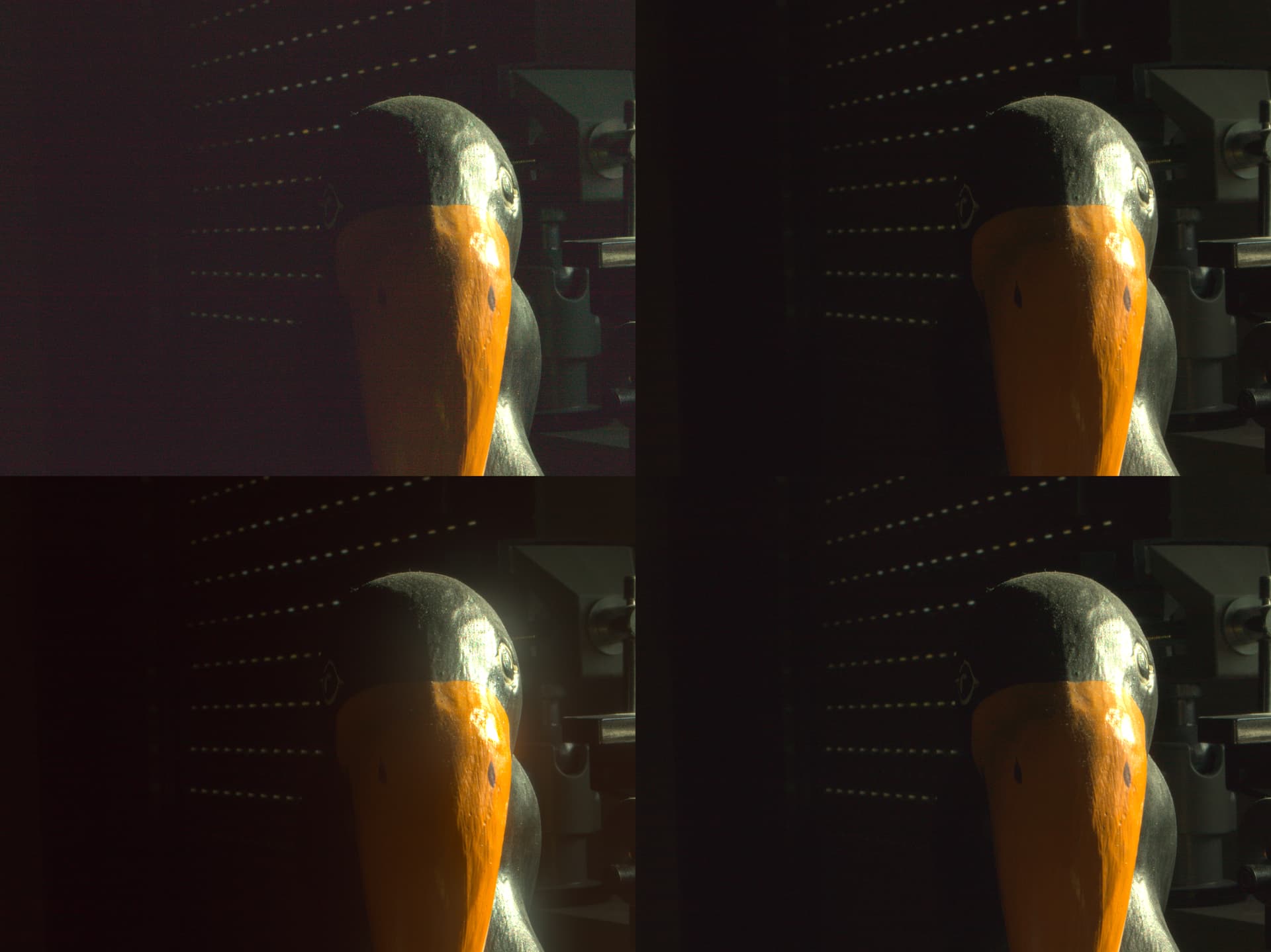
  • Top Left: only the raw data from the two exposures with 0.002 and 0.004 secs were fused together. The resulting raw was than “developed” into the single sRGB image presented here.
  • Top Right: only the raw data of the two exposures with 0.004 and 0.016 secs were fused (the two brighter exposures). The resulting raw was again developed in the same way as the “Top Left” result.
  • Bottom Right: the raw data of all three exposures were fused and developed.
  • Bottom Left: all three raw exposures were individually developed into sRGB (jpeg-like) images and these sRGB images were exposure fused via the Mertens algorithm (that is the classical “exposure fusion” way).

Time for a short discussion: Clearly, the “Top Left” image show noticable noise in the dark areas. The “Top Right” result is better, the best result is obtained in the “Bottom Right” corner. The exposure fusion result (“Bottom Left”) is comparable to this, but it shows some noticable glare effects.

These glare effects are due to the way exposure fusion works and can only be avoided by working directly with raw images. In fact, I created this test example especially to show this effect. However, most of the time, this glare effect is not noticable. Here’s an actual film frame calculated the same way as the test image above:

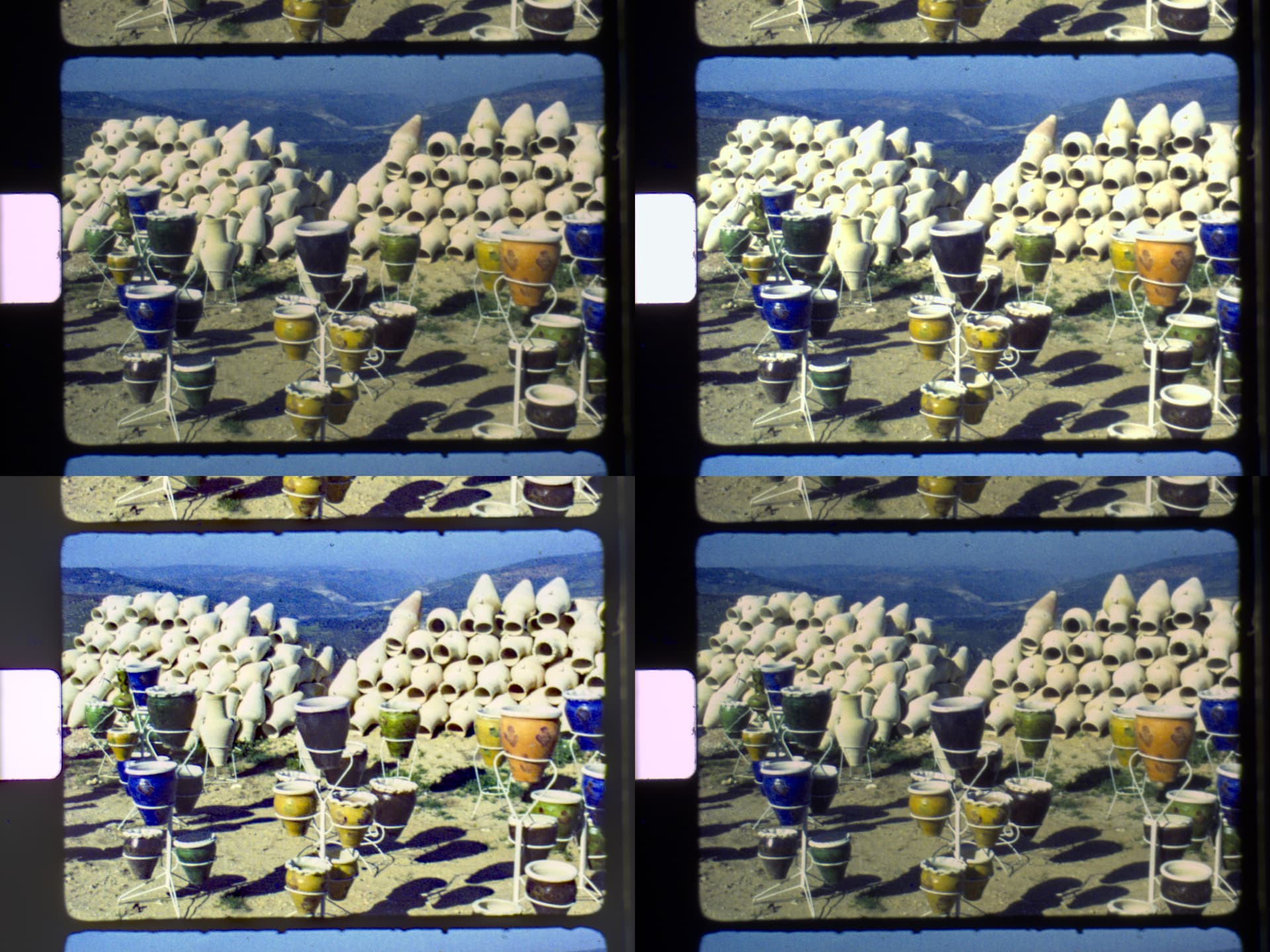
Note that the exposure fusion result (“Bottom Left”) shows more vivid colors and some haze reduction in the far distance. This behaviour is “backed in” the exposure fusion algorithm. But actually, the 3-exposure raw image result (“Bottom Right”) is more true to the actual film frame.

Well, that is my current state of affairs.

At this point in time, I think my old way of doing things, namely capturing several jpgs of a single frame following by classical exposure fusion will give me better results in terms of image quality, as well as capture speed.

So I do not think that I will develop the raw capture stuff further.

Because of the limited dynamic range of raw images (only 12bit), capturing in raw also requires several exposures per frame; while it’s more accurate than exposure fusion of multiple sRGB images, it’s not faster and the visual quality isn’t significantly better.

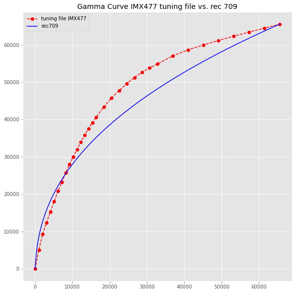
The next goal in this project is to come up with an own tuning file for the HQ sensor (IMX477) which minimics closely the processing I have applied above – in effect persuade libcamera to do the necessary processing for me. There is still a lot to do.

For example, the gamma-curve of the IMX477 tuning file does not follow rec 709 at all, like the following graphic shows:

As noted in another thread, the color matrices (ccm) in the original IMX477 tuning file do not work well either. The problem is probably caused by the way these tuning file were created – there is very little information available about this.

However, I think I succeeded in calculating optimal ccms from a given spectral distribution of the illumination and the camera sensor used (in this case the IMX477).

The “development” of the first image above is based on a D65 illuminant, the second one (the film frame) is actually based on the spectral distribution of my 3LED-setup. The first image uses the stock HQ camera, the second image (the film frame) a HQ camera where the IR-block filter has been replaced.

So my current idea is the following:

  • use the picamera2/libcamera approach to create “jpg” images with a special tuning file, calculated especially for the illumination source of the film scanner.
  • Take 3 to 5 different exposures of each film frame, transfer them to a fast machine for exposure fusion.
  • As I now know, white-light LEDs with a high CRI will give me better results than my current 3-LED setup. So the red, green and blue LEDs of my scanner will be replaced by white-light LEDs. As I could only source Osram Oslon SSL80 with the form factor I need, these will be used. They are not perfect, but listed with a CRI between 90-95.
  • Also, I now know that a previous experiment (the replacement of the stock IR-filter with a better one) actually results in worse color rendering. So the current camera (with a flat response curve IR-filter) will be replaced by a stock camera, employing the standard Hoya CM500 IR-block filter.

Stay tuned…

3 Likes

For me the dynamic range is more a characteristic of the sensor than of the bit depth of the encoding.The dynamic range measures the ability of the sensor to capture details in the shadows without losing them in the highlights. It is not the 12bit encoding but a weakness of the IMX477 sensor that we try to correct with HDR

Regarding the RAW format, I think that it does not bring anything in our case of film scanning
A professional photographer will capture in RAW to avoid all the sophisticated processing that the camera processor can do. He prefers to keep control over his processing and do it himself in the “development” of the RAW. In the case of libcamera these processes are quite basic and can be controlled or disabled so your idea of working on the tuning file seems relevant to me.

To be more precise, if I understood the documentation correctly, libcamera successively applies various algorithms on the image, which determine parameters that are sent to the ISP (except the exposure directly to the sensor) but “in fine” the image comes from the ISP. It is the same ISP as before with MMAL/Picamera so it should be possible to obtain the same image by setting or disabling these algorithms. As you have noticed the most problematic algorithms are the ALSC lens shading and a CCM color correction using AWB and a very dubious tuning file. They were not used before (except for ALSC in a modified version of Picamera), why not start from uncalibrated.json?

Finally our current projects digitize with a limited resolution, the question remains open to know if we could obtain a satisfactory result with the HQ maximum resolution with libcamera, a careful programming and a more powerful hardware like the PI4 (when we can buy it!)

About programming I learned something interesting in a PICamera2 discussion. It seems that in a multithreaded context the Python GIL lock is released when calling a C/C++ library like jpeg encoding allowing real processing concurrency.

Dominque,

thanks for your comments! Here are some thoughts/comments of mine:

Well, the dynamic range a sensor can capture is directly related to the bit-depth the DACs of the sensor are working with. At this point in time, the 12 bit of the IMX477 is not that bad - even high end DSLRs do not deliver much more that 14 bits. The information which the sensor has captured is usually compressed into an encoding bit-depth of 8 bits (jpg, for example). That is, substantially less. That is the reason a lot of people work with raw files: you can recover (by manual tuning) shadow- and highlight-detail which is lost in the usual jpg.

In any case, 12 bit is less than what you might experience when scanning color-reversal stock. It will be sufficient for well-exposed scenes, but it will not be enough for high-contrast scenes. If you use automatic exposure, most of the time things will work out ok - after all, that is what this algorithm is trying to achieve. The disadvantage with autoexposure is that in case of strong changes in the frame’s brightness, autoexposure takes much longer than 3-4 frames. Also, autoexposure will introduce brightness changes in your scans which are not present in the source material. Depends again on your material whether this is acceptable or annoying.

Actually, not really. They are quite comparable to the type of algorithms your DSLR is using…

Well, from an archival point of view, storing the raw data the sensor has captured is the optimal way of scanning old decaying film stock. Not so much from the view of processing time and storage requirements. You will need at least two raw captures with matched exposure times to digitize a color-reversal frame in full fidelity.

Well, of course the CCM was used before. In every camera, you apply red and blue gain to the raw image to obtain a white-balanced intermediate image. These gains are usually chosen for you by the whitebalance-algorithm. From this intermediate image a pre-output image is calculated via the CCM (compromise color matrix), and this part is the most important step to achieve good colors. Finally, a gamma-curve is applied to this pre-output image - this final image with the gamma curve applied is what you get as jpg or png. (In fact, what I described is the most basic workflow. Any color camera, from a cheap USB-webcam to a high-end DSLR features this. Sometimes, work is done in intermediate color spaces, often non-linear lookup tables are employed,etc. But the basics remain as sketched above)

Now, there exists actually a json-file of that type you are thinking of, which is used in camera calibration. However, as it is required by the calibration, there is no color-processing enabled in this tuning file. So the images you will get with such a tuning file are rather disappointing, to put it mildly.

On the other hand, coming up with a real (and good working) tuning file is not trivial. The deficits of the current tuning file are related to this non-trivial challenge. You need proper illumination, precisely measured color targets and a whole bunch of expensive color measuring instruments, for a start.

In case of our film scanning application, in the above list something is hidden which definitely spoils the game substantially: namely the “precisely measured color targets”.

The color targets should be in our case made out of the film stock we are scanning, and it should feature a range of different color patches from which we exactly know the color they should have in the final scan result.

Now, I am unaware of any such target for our Super-8 format, for any film stock imagible. It fact, even for existing film stock, it would be very difficult to produce, and for the film stock we are probably most interested in, Kodachrome, there is no film stock left to produce such a target. So at this point in time, it will not be possible to create such a target.

That is the challenge I was trying to solve during the last months. I think I have found an alternative approach for good libcamera-tuning files.

I have developed a way to actually calculate the basic values in the tuning file directly from the spectral distributions of the light source + the spectral distributions of the Bayer-pattern in front of the sensor (well, the IR-cut filter has also to be taken into account). In fact, the two example images above were created exactly by this approach. In other words: I was able to realize a camera tuning without the need of color checker targets or color measurement devices.

Obviously, the next step is to realize the above processing (which was done in Python) in a way that libcamera itself can do this. At this point in time, I am quite confident that I can achieve this, but it will take some further time on my side until I can report any news on this.

As we have discussed before, the old “mode 2” with 40 fps is inferior to the old “mode 3”, running only with 10 fps at most. The basic bottleneck are here the two CSI-lanes which connect the camera to the Raspberry Pi. Also, the sensor itself has some limitation (which I do not have at hand currently). As far as I know, the compute module features 4 CSI-lanes, which could potentially lead to a speed up - if there would be a new camera PCB which has all four CSI-lanes routed. Quite possibly third-party companies like Arducam might be able to come up with something like this.( EDIT: they actually offer this; however, I doubt the software support is sufficient enough developed to acutally bet on this. They claim a framerate of 4032×3040@30fps for this camera.)

However, I am quite satisfied with the performance of the RP4/IMX477 combo. Who knows what will be available in one or two years? The main bottleneck with my system is not related to the framerate anyway. I need to spent about a second for each frame just for mechanical vibrations and the like to die out, and, due to the design of libcamera, I need to capture about 4 frames for each exposure (instead of a single frame). And I do not think that these points will change in the near future…

Well, that is true, but that trick does not help to substantially to speed things up. Picamera2 actually features already a framework where a simple encoder can be encapsulated into a multi-encoder using 4 or more threads to speed things up with that approach.

Also, it does not help too much in our application scenario, from my experiments. I used this trick (which is actually an old one in the context of concurrent processing in Python) within the context of my exposure fusion algorithm (which is based on C/C++ cv2-routines). In this case, the speedup was substantial, as this algorithm is running on a WIN10 PC with 12 cores. Here, there’s a difference between Python code running on only 1 CPU vs 12 CPUs.

2 Likes

I would agree with the comments by @cpixip regarding the sensor/raw/bit depth.

@dgalland a few comments from my own experience about capturing in 12bit NEFF (RAW with some compression) at 24MP.
JPEG is lossy. Most of the film I converted was 8mm from the early 60s. These typically have wide variations in exposure, even within the same scene (dark/light on the same frame). Additionally, the film dye have faded. What I found is that capturing in 12 bit raw, even with some compression (NEFF of my camera wasn’t lossless), provides the ability to address these issues in post, particularly in regards to color correction to fix faded dye. It also gives the latitude to set the interest exposure in the visual range of the output. Doing so with a JPEG source file generates all kind of quantization and compression artifacts. Worth noting that all the film was being captured with a set exposure (no auto range).
There are alternatives to RAW for the above, such as lossless 16 bit TIFF. But obviously what cameras typically provide is RAW or JPEG.
For me, it was also important to look at any limitations on the workflow. I used virtualdub2 for conversions, and there were some filters that limit the output to 8bit (I think deshaker was one of them).
If one starts with 12 bit, even at single exposure, there is range for adjustments, and one can end with HEVC at 10 bit for stunning reproduction in a typical Samsung TV.
If I was to sketch a new workflow, would love to do at the minimum of 4 exposures per frame (with different illuminant intensities) captured in RAW, apply Mertens, then save as 16bit TIFF for post (TIFF requires less processing to save and read, it does take a more storage space), and output as 10 bit HEVC for the Samsung TV. From what I have, from glass to glass, that is probably the best dynamic range one can get.
Will it be slow, will it require lots of space… yes. But for 3 minutes of priceless content, it is worth every second and every byte.

I’m a new user; first post, hello everyone!

I know it’s been a few months since you mentioned this and I’ve spent all morning trying to catch up on years of all these amazing discussions from everyone here, so I may have missed it, but: have you talked about this new calibration method in more detail anywhere yet?

I would love to hear more about how you were able to accomplish this. I’ve got one of Wolf Faust’s 35mm color targets on Ektachrome which I was hoping might get me in the right ballpark, but my eventual scanning target is about forty 3" reels of old (50’s through 80’s) Kodachrome, so I’ve been hunting around for something that might be a closer starting point, color calibration-wise.

Does your method depend on using the Pi HQ camera? (I grabbed an IMX429-based industrial camera a few years ago, before the Pi HQ was available.)

Thanks!

Great that you joined! Have fun and contribute!

Well, all of this is still a work in progress. I too ordered an Ektachrome slide from Wolf Faust - thinking of using this for the calibration of my setup. However, two things stopped me in this endeavour - first, I could not figure out a sensible way to scan the 35mm slide with my camera imaging only the much smaller Super8 format, and second: I am not really interested in Ektachrome, as my material are brands available in the 70th or early 80th of the last century. That is, mainly Kodachrome and (the comparable) Moviechrome, plus a assortment of non-name film stock (Fuij, etc).

So I opted for solving this from a totally different approach: just simulate the camera (mainly the sensor with its Bayer-filter + the IR-blockfilter) together with a simulated light source to come up with the appropriate color science. As a test, I created a tuning file for the IMX477 sensor build into the Raspberry Pi HQ camera, only to discover that the numbers I got where close, but different from the standard tuning file. Nevertheless, I published the new tuning file (it is available in the latest Raspberry Pi release as “imx477_scientific.json”) and invited people to test it. The feedback I got so far was modest, but positive.

So I think I have a working technique to approach the color science of a certain setup without the need to actually take images of a color checker. How far I can push this in our application (film scanner) remains to be seen. What I have achieved so far is getting the color science given a certain sensor and illumination. What is missing at this point in time is how to treat the color science of the film stock in question - I simply do not have enough data for Kodachrome, for example.

Indeed. The color science put into the imx477_scientific.json file depends on the specifics of the sensor used, the imx477, the IR-block filter used (a Hoya part), the lens used (however, currently modeled as “ideal lens”) and the illumination (mostly daylight, with a switch to tungsten below about 4000 K for the imx477_scientifc.json). If any of these variables change, say the illumination is not “daylight”, but a white-light LED, the numbers in the tuning file will change. Specifically, the ct-curve the AWB is using, and in turn the ccm’s for the various color temperature will have different values.

1 Like

Everyone here is so responsive and helpful so far! I feel like I’m going to seem slower just because it usually takes me a few “lying in bed” or “standing in the shower” type of events to assemble the pieces of whatever puzzle I’m working on in my head. :rofl:

Ha, ha! I had been wondering the same thing, down to having several half-finished sketches of something that I might be able to swap out with the 8mm gate to take (what, a little more than 16?) small exposures of the 35mm slide and stitch them together in software afterward. That led down the path of worrying about having a uniform enough backlight for the stitching… and it always seems like the rabbit holes never end. :sweat_smile:

It sounds like your direct results so far are only for the IMX477, but from what you described–as long as the curves are available (or measurable) for a given sensor–the method itself should be broadly applicable to just about any setup, right?

Using the expected, virtual response from the datasheet is definitely a cool idea. I’d be curious how much variation there is in the response from sensor to sensor. I know when you’re learning electronics, there are certain quantities you can trust (say, the resistance of a 0.1% resistor at a known temperature) and others that they teach you might vary by a wide range from unit-to-unit compared to what’s on the datasheet, like the β value of a BJT. I wonder where sensor response falls in that continuum?

I guess real world experience with calibrating my monitors and cameras over the years tells me it should be close enough that your method has a good chance of being useful. (The color profile that Adobe has shipped for each one of my dSLR’s over the years has always been rather close to my own measured values, so the variability between sensors can’t be that large.)

Very interesting. Thanks again for sharing!

:joy: - that sounds very familiar…

I think so. Provided the published data is real, not beautified by some marketing guy. I measured the transmission of the Hoya IR-block filter by myself - this is rather easy because you can take it out of the camera and throw it in a spectrograph, but for the spectra of the Bayer-filter, I have to trust what is published. Jack Hogan describes on his blog a way to measure this with an easy setup - that’s one of the things I want to try in the future.

There certainly will be a variance. But I suspect that it will only be noticeable by measurements, not by the human eye. At least the several HQ cameras I tested did not show any visual deviations in performance.

Yes, I think so. But I am still researching this. Not 100% sure that my approach and calculation are correct, I still need to do more testing. The feedback I got so far was ok, no major objection from the people testing the “imx477_scientific.json” tuning file. Currently, my mood is that I trust my approach more than the classical approach (imaging color checker boards at various color temperatures and calculating the color matrices (ccms) from these calibration images) - but that might change with time…

Here’s a comparision of the ccms obtained with the classical approach (taken right from the “imx477.json” tuning file and the new approach (data from the “imx477_scientific.json” tuning file:

While the matrice values are close to each other, the variation of the ccms in the new tuning file (blue curves) is much smoother than the ones obtained by the classical approach (red curves). The little kink of the blue curves around 4000 K is caused by switching from tungsten illumination to CIE standard illuminant D for higher color temperatures.

This is going way overboard, but you could sort of reverse which side the Bayer filter is on. My profile picture is from one of my earliest experiments before I’d found any information online and was still going down lots of my own blind alleys. Those are the standard Wratten RGB tricolor separation filters, lens-filter sized, on custom machined/threaded aluminum tubes, lit using the highest CRI LEDs I could find at the time (YujiLED, I believe).

I mentioned it in the other thread, but my original reason for choosing monochrome was to get away with buying a lower resolution camera (4k was harder to come by in 2015! The RPi was still on the v1 camera, etc.) without losing so much information to the Bayer filter. So I found the Wratten filters that had the same response as your typical camera sensor Bayer filter and… well, I never really solved the problem of how I was going to get these giant tubes to all point in the same direction as the image plane. I think at one point I was envisioning a stepper-driven rotating table to physically move which of the three lights was in the optical path. I’d never heard of an integrating sphere at the time.

But at that point, once you have the filters separate from the sensor, they would be easier to measure for your purposes… it’s just everything else that would be harder. :rofl:

It’s all very embarrassing to admit now because it was a silly idea. I didn’t know anything about projectors, mechanics, electronics, optics, or much of anything. The little PCB on the back of each tube was my second circuit board design ever and the tubes themselves were my very first machining project on the micro Sherline lathe I’d picked up the year before. I’m a software engineer by trade and the reason it’s taken so long to plan what I want to build is because I’ve been sitting down to learn each subject before I proceed. I’m halfway through my third electronics textbook in three years. :grimacing:

(I picked that image for my profile because it’s a good reminder of how far my understanding has come along and to remind myself that I make mistakes almost constantly.)

The sharp, abrupt changes in the red curve seem obviously incorrect. Like someone used an automatic process to generate them (with incorrect settings, bad data acquisition, or serious overfitting) but then didn’t actually look at the data before publishing it. That’s almost the kind of comparison you’d want to send to the manufacturer (or whoever made imx477.json) and report it as a bug.

I’m more willing to trust yours just on the merits of it having dramatically smoother curves. :smile:

Well, these files come from libcamera’s approach, adapted by the Raspberry Pi foundation for their hardware. I think this is the first time in history that camera performance got so accessible to common people.

Camera calibration is a challenging thing; you need expensive measurement devices and lot of other equipment, most notably a bunch good lights with different, clearly defined color temperatures.

Taking that into account, the imx477.json is not that bad. It does however contain a lens shading section with data, even so the HQ camera is sold without a lens - that is a little funny. That this section is present (and fixed) in the tuning file is a design choice made by libcamera. Something like this certainly makes sense if you are concentrating on mobile phone cameras with their fixed lens, but is funny for camera sensors with interchangeable lenses. But - things are rapidely evolving, so all this might be improved in the future.

Ahh!! Even more reason to be suspicious of it.

Unless the lens shade data is for some calculated, generic amalgamation of a hypothetical “average lens” (which is a stretch when you consider the staggering variety of projects you find Raspberry Pis hiding in), it’s starting to sound like someone was indiscriminately copy-pasting data from other profiles until it looked good on their end.

So, thanks one more time for bringing some sanity to the community with your imx477_scientific.json!