Pi HQ Camera vs DSLR image fidelity

which has been discussed here on the forum as well :wink:

Oh, you’re right. I remember the bug!

First: did you change your illumination source between captures?

Yes and no. It’s the same lamp and diffusing sheet, but the lamp was further away and not semi-encased as in the projector. But that’s interesting. I thought you could see the structures less because I didn’t get the focus right.

The sprocket hole should have exposure values of 100% in the raw file, nothing less.

Makes sense… yup. I’m used to all the little helpers of the DSLR and am only halfway finished with adding a little histogram feature to my script. I should probably try out one of the more sophisticated scripts linked in these forums, but I like tinkering first :slight_smile:.

the digital gain stays at 1.0. You do not want any other value.

I set gain to 1.0 and exposure time to a fixed value, but no matter what I set, digital gain is something above 1.0. How do I know which exposure values are native to the Pi Camera?

Please note that the .dng-files the HQ/Schneider combo would produce can be read directly into DaVinci Resolve.

It’s the same workflow with the Canon :slight_smile:. MLV splits into individual dng-files which I can use directly. Similarly, I’d use Adobe DNG converter on the Pi files, just to reduce their footprint (lossless compression).
How do you guys manage those big files, anyway? One 30 Minute film would have 800GB of data (or around 500 if run through Adobe).

This is not a discovery, but the result of optical calculations!
Distance lens (lens optical center) image 50*1.0858+ 50 = 104.29

Thanks for this immensely useful calculation! I’ve been trying to figure this out on my own and couldn’t find anything succint enough for my monkey brain.

Small edit: I’ve been trying to apply this formula to other setups, but can’t relate some of the values. Is it both times the lenses focal length?

I’m using a slightly lower resolution sensor than the HQ camera, but after combining the separate raw RGB and IR exposures, they end up just shy of 17MB for each frame so the amount of data is in the same ballpark.

Since I knew my own collection of reels was around 4 hours of footage–and I don’t know if this is a good answer or not–I just bought a pair of 12TB hard drives and have them set up in a RAID 1 configuration in my PC so everything is duplicated for safety. It’s kind of wild how cheap “spinning rust” has gotten compared to any other kind of flash or optical storage.

While working with the frames I copy them over to a fast SSD (otherwise it’s painfully slow in the editor!) but most of their “cold storage” time is spent on the pair of HDDs. (As a final safety precaution because I’m paranoid, I keep the file hashes for each frame and confirm them whenever data is moved between drives.)

1 Like

You might want to read here (section “Image formation”) for more information. Actually, the German version is explaining things better. In any case, in the real world, lenses do have principle points and other properties which might throw such simplified calculations off the track. Nevertheless: if you want a 1:1 magnification, the general rule of thumb is that you simply place the object in a distance equal two times the focal length and the sensor in the same distance as well. That gives you 1:1 imaging.

Specifically, for the standard setup of a 50mm Schneider lenses paired with an HQ sensor you place the object in 2*50mm = 100 mm distance. Also, you use the same 100 mm distance between lens and sensor. Again, that is not exact and will only give you a ballpark to improve upon.

That was what was quoted above and that’s what I am using in my setup as well.

Well, get yourself a few TB of fast SSD. And make sure your computer can handle the data rates.

Note that “lossless compression” requires additional computations when reading the files back from disk. Not much of a hassle if you have a fast computer, but it may slow down things when editing.

Another approach would be to reduce the size of the image data you are working with. Normally, I take the 4k raw files from the HQ sensor and pipe them through DaVinci. The developed raw files are scaled down to some reasonable resolution for my project, say 2400x1800 px for HD target resolution, and than rendered out as either linear .tif or .png with 16 bit depth. This format is what I use as basis for further processing, seldom looking at the original raws again. You can compress .tif and .png data as well; at least my hardware is able to handle that data within DaVinci in real-time. But I usually do not bother, in exchange of a slightly larger disk space requirement.

In addition, I simply use sufficiently fast storage (Samsung T7, 4TB for example) + the ability of my NLE program to produce proxies for post production work. You need to make sure that your USB3 ports and USB3 cables are both able to support the highest speed these disc are able to work with.

Well, you have triggered old memories here (which I was obviously trying to forget…). Citing myself,

" Another important deviation from the old picamera-lib is the handling of digital and analog gain. In the new picamera2-lib, there is actually no way to set digital gain. As the maintainer of the library explained to me, a requested exposure time is realized internally by choosing an exposure time close to the value requested and an appropriate multiplicator to give the user an approximation of the exposure time requested.

An exposure time of, say, 2456 is not realizable with the HQ sensor hardware. The closest exposure time available (due to hardware constraints) is 2400. So the requested exposure would be realized in libcamera/picamera2 by selecting: (digital gain = 1.0233) * (exposure time = 2400) = (approx. exposure time = 2456)."

and

“One approach to circumvent this is to choose exposure times which are realizable hardware-wise and request this exposure time repeatably (thanks go to the maintainer of the new picamera2-lib for this suggestion), until the digital gain has settled to 1.0. For example, the sequence 2400, 4800, 9600, etc. should give you in the end a digital gain = 1.0. And usually, it takes between 2 and 5 frames to obtain the desired exposure value.”

I think one way to figure out which exposure times are directly realizable with the hardware is to request a certain exposure and monitor the digital gain which is returned in the metadata. Due to an automated process running in the background of libcamera, you will need to capture at least 10-20 consecutive frames before you read out the value of the digital gain. If it’s close to 1.0, you have found one exposure time you are after.

Note: this was the status about 2 years ago. There has been work done on this, so things might have changed. Never bothered to check again - libcamera and picamera2 are technically speaking a mess and overall a rather bad design. And the libcamera people as well as the RP guys tend to change things happening under the hood without much information towards the user. That’s why I am very hesitant updating these two software packages once I have a running/working system.

Let me note that questions about picamera2 can be posted here. The maintainer of the picamera2-library is rather responsive and helpful. Also, searching the “Closed” issues you might discover some useful information.

Update: I had a discussion with David Plowman, the maintainer of picamera2, about the current state of affairs (Sep '24). According to him, DigitalGain is only applied “to the fully processed ISP output”. It is not applied to the raw output. So DigitalGain is relevant only if you store rec709-like images as .jpg or .png, for example. In case of linear raw files (.dng), only the AnalogGain gets applied. So, if you are working with raw files, no need to worry about the DigitalGain-value. And of course, you should set AnalogGain = 1.0 for the lowest noise level.

Well, get yourself a few TB of fast SSD.

I thought so, too, but I’d wager there’s about 10 hours of material lying around here, so I’m going to run out of space fast :-).

I’m going back and forth between the two cameras and I think it’s mostly the file size that’s keeping me from simply using the HQ cam at full resolution. A few questions came up.

So far I’ve only been thinking about using Adobe DNG converter as it reduces file-size to about 2/3 (lossless). It also has a lossy compression feature that unfortunately doesn’t clarify which type of compression it uses (JPEG or JPEG-XL), but resulting bit-depth is 8, so I assume it’s JPEG. The differences between both are… detectable if you overlay them in Photoshop with a difference layer, but even then you’d have to look closely. Unfortunately DaVinci can’t open the files for some reason.

Now I’ve tested slimRAW, and by e.g. using their “lossy VBR HQ” setting it reduces file size to about 6 MB, preserves 12-bit color depth, and the images look pretty much indistinguishable from their respective originals. The problem with slimRAW: It refuses to read Pi HQ DNG natively - I have to put the files through Adobe DNG Converter first. Even then it only picks up the full-resolution ones, and afterwards the files will only open in DaVinci…

I couldn’t find anything on slimRAW on the forums and nothing anywhere else regarding possible issues with slimRAW and Pi Camera files. Obviously there’s something that the Adobe Converter does that makes the Pi DNGs readable with slimRAW, but I don’t have the knowledge to know where to look for possible differences. Are there any options at all to writing DNG files from Pi Camera RAW data?

Update: I had a discussion with David Plowman, (…) about the DigitalGain-value

That’s going to save me some tinkering. Thanks!

I personally would not do it. It takes time to compress the data, it takes time to extract the data again. You only gain 1/3 of disk space.

Never do something like this. As you noticed, it kills your image quality.

Because the .dng-files created by picamera2 are kind of non-standard (only one CCM instead of two CCMs in a standard .dng)

Yes there are. In my picamer2-based software, I actually create a .dng directly in memory, send it via LAN to a faster, bigger PC, where it is simply received and stored as it is directly as .dng-file. Once scanning is over, I simply drop all these .dng-files as a single clip directly into the media page of DaVinci. That’s all. Direct HQ/RP5 to DaVinci pipeline. Nothing could be easier. Details are distributed here on the forum in various threads; if I find time this weekend, I’ll write everything together into a single thread.I think @dgalland’s software is doing a similar thing.

Never do something like this. As you noticed, it kills your image quality.

But… does it? I agree that Adobe’s lossy algorithm isn’t an option because it reduces bit-depth to 8. But slimRAW doesn’t. I am able to see the differences in pixel arrangement when I look at these images at 500% zoom, but is that really relevant?
Granted, I don’t have any proper scientific ways to compare those three images, so you might convince me otherwise.

https://drive.google.com/drive/folders/1iT-17EFZl-d7H4SXIUENX-OIf7-ZEpev?usp=sharing
The ones named “Timeline*”. It’s tif, because I had to load the frames into DaVinci, then did the same basic color grading on each, then exported them again.

Because the .dng-files created by picamera2 are kind of non-standard (only one CCM instead of two CCMs in a standard .dng)

Is there a way to save a “standard” DNG, though? (I really wish I had more knowledge about these things. It’s not easy to catch up).

I actually create a .dng directly in memory, send it via LAN to a faster, bigger PC, where it is simply received and stored as it is directly as .dng-file.

Do you mean a raw data? Or is it already a dng before it’s sent over? How does the receiving PC store it as DNG?
Does the PiDNG library by itself have more options available? The examples are rather lacking…

Once scanning is over, I simply drop all these .dng-files as a single clip directly into the media page of DaVinci.

I wouldn’t do it any other way.
…Only, maybe, lossily compressed :grin:

Do you mean a raw data? Or is it already a dng before it’s sent over? How does the receiving PC store it as DNG?

In my software, using functions from the picamera2 library, a .dng file is generated which is then sent via LAN to the main computer whose job is simply to save it to disk so that after the capture phase, post-processing can be carried out, for example with DaVinci.

I attach the python function that carries out these operations:

Take and send a dng file.

def takeAndQueueDng(self, imgflag):        
    
    # The new exposure time is stabilized.
    if not self.cam.autoExp:
        self.stabExpTime(self.cam.exposureTime)
    
    # Raw image is captured.
    request = self.cam.picam2.capture_request()
    
    request.save_dng("file.dng")       
    
    request.release()
    
    # Sending flag.
    self.imgSendThread.imgflag = imgflag.encode()
    
    # Sending dng file.
    with open("file.dng", "rb") as dngFile:
        self.imgSendThread.stream.write(dngFile.read())
    
    # Sending the exposure time.
    self.imgSendThread.exposureTime = self.cam.captureMetadata().ExposureTime
    
    # Thread start.
    self.imgSendThread.event.set()
2 Likes

Well, of course. Any lossy compression algorithm is just that: lossy. Whether you will notice or not depends on the circumstances.

The simplest approach to smaller file sizes, faster processing and irrelevant image loss is often overlooked: reduction of image size. For example: a HQ-sized .png (4048 x 3023 px) might come along with 67MB of storage; the same image scaled down to 2400 x 1800 px only requires 23 MB storage space. And that’s a resolution which is for most workflows a sufficient resolution for S8 material.

Well, there is indeed a spec by Adobe. Problem is that it is so complicated that no-one implements it to the full - save maybe Adobe and other software based on Adobe’s implementation.

.dng is intended to be an intermediate/universal raw format, freeing the user from all the individual implementations of the various camera manufacturers. But you have to “translate” your cameras original format into the .dng-format. This is what Adobe’s raw converter is doing. So, that’s the “standard” way of creating a .dng-file.

In doing so, the converter needs to translate the camera’s metadata into the .dng-format’s metadata tags. How that is exactly done is not that clear. Specifically, a .dng-file contains color science information. How this gets translated into the .dng-color information is dependent on the camera model and, up to my knowledge, undisclosed.

The usual .dng-format contains two color matrices, corresponding to a cold and a warm color temperature. In addition, also the color temperature at the time the image was taken is can be interfered from the metadata contained in a .dng-file. Any software developing the raw data is expected to use the image color temperature and interpolate the real color matrix from the two color matrices located at the far end of the color temperature scale.

That’s the usual/“standard” .dng-file. There are other, more complicated forms of color metadata defined in the Adobe standard, but that’s not relevant here.

The software used in picamera2 is a free software implementation which just contains as metadata a single color matrix - namely the one the camera thought was appropriate at the time of picture taking. That is: either calculated by the AWB algorithm, or specified by you as a user, setting red and blue gain.

While this format is perfectly ok - it is in a sense even preferable, as it is not necessary to interpolate - it might cause trouble in software assuming to get two color matrices for interpolation.

In addition, the free software solution utilized in picamera2 set some other tags a little bit wrong and that is also a potential source of software refusing to process .dngs directly from the HQ sensor.

The important thing is: DaVinci understands the HQ/picamera2 .dng-format correctly. I doubt that a picamer2-dng file run through Adobe’s raw converter gives you the same color science as the original .dng. But: I have not checked that, as this additional conversion step does not help in any way. At least not in my workflow.

@Manuel_Angel already posted some code on how to store such a picamera2 generated.dng-file directly. As mentioned above, I may not have time to gather all the necessary information until next weekend.

3 Likes

Sorry to reply here with no real info to add to actual discussion.
I just have to emphasize to all of you who share your knowledge here, that it is tremendously appreciated. All the bits and details make for a really interesting read, and even though it’s sometimes hard to digest all the details, it is much appreciated.
Thank you all! :pray:

@cpixip it would be really helpful to others (me at least) if you could gather all the details of your process, but I know this is no quick task.

There’s so much info on this site, that I get lost in “what is the current best way to go”, “what is just a matter of opinion” and so on, but still interesting to read nonetheless.

2 Likes

Well, this thread started out as a comparision between the Pi HQ camera sensor and a full-frame DSLR. Let me try to summarize some things about the HQ sensor and the associated software environment.

Over the years, the Pi guys have offered several different types of sensors and quite different software libraries as well. In summary: do not bother with any of these sensor types other than the HQ sensor and: be aware of some weird things happening under the hood of the software (libcamera/picamera2). I will try to elaborate on all these things.

S8 footage

Before we go further, let us remind ourselves about our target to digitze: we are considering only S8 color-reversal film stock.

The camera frame of S8 footage has a size of about 5.7 x 4.3 mm. Though usually, a slightly wider frame is exposed. Depending on the film stock (Kodachrome, Agfachrome, etc) and the type of camera used in the old days (Leicina, Bauer, Chinon, etc) , the effective image resolution might vary from less than 480p (SD) to 1080p (HD). The typical dynamic range of a well-lid scene is around 11-12 bits with color-reversal film stock, whereas strong contrast scenes can exceed 14 bit dynamic range.

The Hardware

The first camera the Pi guys introduced was the V1 camera, followed by V2 and V3 versions. All of these cameras are based on mobile phone technology and should be avoided for telecine work. The main reason: the sensors used in these cameras feature a microlens array which is matched to the focal length of the attached lens. If you swap that lens with a lens of different focal length (which you have to for telecine work), the mismatch creates a magenta color cast in the image center which is not recoverable.

So in the end, there only are two units available from the Pi guys which might be of use for scanning S8 film. Both types (GS/HQ) do not come with a pre-attached lens, instead, they feature a standard C/CS-mount.

The GS (global shutter) sensor is nice, but the maximal resolution of 1456 x 1088 px is not really high enough to scan the resolution of S8 film stock well. So the only option available for a decent telecine within the Pi offerings is the HQ sensor.

The HQ sensor, more correctly the IMX477, was developed by Sony for consumer camcorder applications. Think of the typical HD camcorder which is able to grab occationally also slightly higher resolution still images. Clearly, at that level, we are not at the end of the line with respect to sensor quality. DSLRs come with much larger sensors, like APS-C or even full-frame sensors. Especially the noise characteristics improve dramatically with larger sensor sizes.

The HQ Sensor

The HQ sensor features a maximal resolution of 4056 x 3040 px (let’s call this 4k) as well as lower resolution modes. Since the HQ sensor uses only 2 of 4 possible CSI-lanes, the 4k mode can only deliver maximal 10 fps.

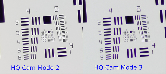
There are lower resolution modes available which deliver faster frame rates, but: do not use them. Especially the 2k mode (in the image below labeled “HQ Cam Mode 2”) uses a badly designed scale-down filter, combined with some annoying sharpening. If you want to work at the 2k res, operate instead the HQ sensor at the 4k mode (labeled “HQ Cam Mode 3” in the image below) and scale down to 2k.

To really see the differences between these modes, view this image

at full size.

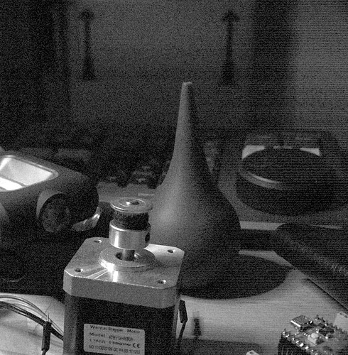
As mentioned above, the HQ sensor is of the “camcorder” quality. Which means that the noise behaviour is far inferior compared to an APS-C or full frame sensor. In addition, various people have noticed that there is obviously some noise processing ongoing already at the sensor level. This results in funny horizontal noise stripes, with increasing noise intensity from the left to the right side of the sensor.

Here’s my attempt to visualize this:

Shown above is the green channel of a severly underexposed image, pushed 6 EVs up to make that noise/image more visible.

If that noise structure bothers you, you better switch from the ~ 50€ HQ sensor to something slightly more expensive. In reality, it probably does not matter to much, as the film grain of S8 footage will cover up the sensor’s noise.

Now, looking at the dimensions of the S8 frame (5.7 x 4.3 mm) and the HQ sensor (6.3 x 4.7 mm), one can notice that they are very similar in size. So, allowing a little overscan area, one arrives at an approximately 1:1 imaging setup. This brings me to the next section.

The lens

First of all, a 1:1 imaging setup is probably the simplest one to realize. In the thin-lens approximation (I come back to this later) you get a 1:1 magnification if you place the object two times the focal length of the lens away. To get the object sharp on the sensor, you need to position the sensor on the other side of the lens at the same distance away, namely two times the focal length of the lens.

Now, real lenses are a little bit more complicated than thin lenses. For starters, they have principle planes and all that. So this arrangement will only yield you an approximation for further refinement.

Another thing one has to consider is the design range of the lens you are using. Typical photographic lenses are optimized for the imaging of objects rather far away. Simultaniously, the sensor is very close to the lens, about one focal length. Clearly, our 1:1 setup with its lens-sensor and object-lens distance of two focal lengths is not matching this design.

However, there is a breed of lenses which has more closely matching design ranges: enlarger lenses. As I operated in the last century my own color lab and still had a bunch of different Schneider Componon-S lenses in my box, this was my obvious choice. Specifically, the 50mm/2.8 - which is easy to get on ebay, for example. Of course, other enlarger lenses are also a valid options.

Now, every lens has an interesting behaviour with respect to the f-stop value. For ease of production, lens surfaces are usually manufactured as spherical surfaces. This is however not the optimal shape. Especially the outer regions of any lens tend to screw the quality of your image. At first sight, there is an easy solution. Just close the aperature (that is, work with higher f-stops) so only the “good” center parts of the lens(es) are used.

This is indeed a working solution, up to a point. If you change the aperature of the Schneider 50 mm from the largest value of 2.8 to, say, 4.8, the image gets less blurry.

But: the is another process working here which spoils that fun. Light is basically a wave phenomen, and if you close the aperature too much, diffraction effects will start to appear. That is: closing the aperature further makes the image more blurry again. Continueing with the Schneider 50 mm, at an f-stop of 8 diffraction starts to degrade the image.

So there is a sweet spot somewhere in the middle of the f-stop range of your lens. Where that specific sweet spot is located depends on your setup. For example, in my scanner setup, it is difficult to align the sensor’s surface really parallel to the film gate. I usually end up with a slight misalignment. So I tend to work with a slightly larger f-stop value than the optimal one, as this gives me a larger depth of field.

Usually, aperatures are also used to regulate the amount of light falling onto the sensor, that is, the exposure. Note that this topic is of no concern in our application. The f-stop is solely selected on the basis of maximal sharpness. Indeed, the exposure should never be adjusted with the f-stop of the lens. Adust instead your light source (if possible) or the exposure time of your sensor.

The Software

The HQ sensor can be handled with various software approaches. By far the easiest way is the libcamera/picamer2 combination, which uses Python as programming language. And I say this as an old C/C++ programer…

Note that libcamera as well as picamera2 are constantly evolving. Picamera2 is still labeled as “beta” and probably will stay in this state for quite some time. So be careful when updating the libraries or your operating system: you might end up with a non-working scanner.

The design goal of both of these libraries is to mimic for the average user the performance and ease of use, similar to mobile phone cameras. Putting that differently: a lot of automatic algorithms are working in the background, quietly adjusting things for you. That’s great if you do not exactly know what you are doing, but somewhat disabling if you know.

Specifically, you will encounter the following challenges:

  • there are things you will never be able to switch off in software. An example is the on-sensor defect pixel correction (DCP) which you can only influence via the command line, out of program scope.
  • other things you are not able to change via software include things which you only can influence by editing the tuning file for your sensor. An example is the ce_enable parameter in the tuning file. Setting it to zero switches off an automatic contrast algorithm running in the background.
  • other things you can set and modify within the picamera2 context, but sometimes the soft- as well as the hardware makes educated guesses in the background about what you really want to achieve. An example is the resolution the sensor is operating at. You might think you are requesting the 4k mode, but picamera2 might decide instead that the 2k mode is more appropriate. Something like this might happen if you operate at 3k - instead of switching to 4k and scaling down, you might end up in operating at 2k blowing up this resolution to 3k. Obviously something one wants to avoid in a telecine application.
  • finally, some settings have side effects, occationally only on certain hardware. For example, the RP5 which works by default in a “visually lossless” raw format. That’s fine if you only want to store .jpgs or so, but it spells desaster if you want to save the original raw data of the sensor. In this case, without telling you, the lossy compressed raw data (which is inferior to the sensor’s original raw data) is uncompressed and saved. Nobody will tell you, except that your program takes about an additional second for this step…

Well, more on all of that later in this post. Before that, we need to look at the various output formats one can work with.

What to capture

Most of the well-exposed color-reversal S8 footage has a dynamic range of about 12 bit. That fits nicely with the maximal dynamic range of the HQ sensor which is also 12 bits. But beware: there are also modes available which operate only at 10 bit, and the RP5’s default mode (the “visually lossless” one) works only in 8 bit, albeit non-linear encoded. You certainly want to make sure that you are operating at the highest dynamic range possible, that is 12 bit.

While 12 bit works ok for most footage, high contrast scenes exceed that range (that depends mainly on the film material; Kodachrome is especially challenging). One way to counteract this is to capture actually not one, but a whole stack of several different exposures from each single frame, from very dark exposures (for capturing the highlights) to very bright ones (for capturing structure in the dark shadows). Before we go into technical details, let’s fix some nomenclature:

  • RAW: that is the raw data as directly recorded by the sensor. Four color channels, Red, Green1, Green2 and Blue. For the HQ sensor, this kind of data has a bit depth of 12 bits. The data is linear with respect to the number of photons received by the sensor. Without further processing (“development” by a raw converter), it is not viewable by a human observer.
  • LDR: this is short for low dynamic range image. It has a bit depth of only 8 bit (or 16 bit) and is displayable on a normal computer screen. In other words, it is viewable by a human observer. To achieve this, some “color science” and at least a contrast curve (say, rec709) needs to be applied to the raw image from the sensor. An LDR features only three color channels, namely red, green and blue. You will get this from libcamera/picamera2 if you request/store a .jpg or .png format.
  • HDR: this is a high dynamic range image. A HDR is usually encoded in a floating point format and thus has an unlimited dynamic range. It is usually neither displayable on a normal monitor, nor viewable by human beings. For this, a tone-mapping operation has to be applied, which converts the HDR into a LDR. Note that in normal internet talk, an LDR created via tone-mapping from a HDR is often also called a “hdr-image”; well, it is not.

How to capture

In the early days, there was actually no way to capture any raw data from the Pi hardware. You could only capture LDRs as .jpg or .png. Remember, such data has a contrast curve applied in order to squeeze the image information into the limited dynamic range of 8/16 bit. Because of this, highlights were blown out and texture in the shadows gone.

So at that time the choice was clear: one needed to capture a stack of LDRs with different exposures and combine them afterwards. In fact, once you have such an LDR-stack, there are two quite different options for further processing: Debevec’s way and Mertens’ way. Both are available within the opencv library (though I work with my own implementations):

  • Debevec’s way: here, the LDR stack gets analyzed in order to recover the gain curves your camera applied to the original RAW sensor data to create your LDRs. Once that task has been achieved, the stack of LDR images can be remapped back to something similar to the raw values your sensor recorded. Each individual LDR covers only a certain band of intensity values. However, by appropriate combination, the full dynamic range of the original frame can be recovered. In principle, you are unlimited with respect to the dynamic range the computed HDR can represent. Of course, you need to convert (squash) this huge dynamic range into a LDR for creating your output video. This process is called tone-mapping and there is an abundance of different algorithms available for this. The main reason: it’s not that trivial to do this.
  • Mertens’ way, also called “exposure fusion”: Here, by a process imitating how the human visual system is working, the LDR-stack is directly transformed into an output LDR. There is never a HDR recovered in this process. In essence, exposure fusion is done by local contrast adaptions. As it turns out, this can in fact even enhance some footage (bad exposure by the S8-camera, for example). A further advantage: from the output LDR of the exposure fusion algorithm you can directly go on to create your digital copy of the S8 footage.

There is however a slight drawback to these approaches. Both operate indepently on each of the color channels. Especially within the exposure fusion context (Mertens) it is difficult to get the colors right because the independent contrast equalization operates and changes colors locally.

Now, as the libcamera/picamera2 software evolved, the possibility of capturing RAW data surfaced. Initially, and even today, the implementation is not 100% correct, but at the time of this post (Sep 24), it is usable. Specifically, the .dng-files created by picamera2 can directly be read by DaVinci Resolve.

Two issues remain when working with .dng-files. Both are related. For starters and as discussed above, the noise of the tiny sensor is noticable. However, especially old S8 filmstock (for example Agfachrome from the seventies of the last century) has such a strong film grain that the noise of the HQ sensor becomes irrelevant. More so if you employ spatio-temporal noise removal - which I do, as I am more concerned about the content than the appearance of old S8 footage. Besides, even without spatio-temporal noise processing, the noise of the HQ appears mostly in rather dark image areas. As these areas end up in the final video anyway as rather dark areas, the increased noise there is barely visible.

So - at this point in time, I would recommend capturing the footage as .dng-files. While working with multiple exposures has its merits, the additional amount of time needed for the various captures, including additional software processing required (you might need to align the various exposures before fusion or HDR calculation because your camera or film has moved a little bit during the different exposures) does not give you such a great advantage in terms of quality that capturing LDRs outperform the ease of working directly with RAW data.So, it’s now time to examine the little traps hidden in working with raws…

Capturing RAWs - Example implementation

As indicated above, there are some things to consider when working with RAW data. The RAW format which the picamera2 lib is delivering is based on Adobe’s .dng-standard. This is a spec for a universal raw format, intended as an alternative to different camera manufacturer’s proprietary raw formats. Accordingly, it is a rather complex format. It features information about the color science of the camera as well as possibly other information, lens distortion and other stuff. A raw developer software should be using all of this information to derive a developed image from the dng.

The picamera2-implementation of the .dng-writer works more on the simple side of things.

Here’s an example of all the data hidden in a picamera2. .dng-file:

---- File ----
File Name                       : RAW_00022.dng
Directory                       : G:/capture/00_RAW
File Size                       : 24 MB
File Modification Date/Time     : 2024:05:25 08:25:06+02:00
File Access Date/Time           : 2024:05:25 08:25:06+02:00
File Creation Date/Time         : 2024:05:25 08:25:04+02:00
File Permissions                : rw-rw-rw-
File Type                       : DNG
File Type Extension             : dng
MIME Type                       : image/x-adobe-dng
Exif Byte Order                 : Little-endian (Intel, II)
---- EXIF ----
Subfile Type                    : Full-resolution image
Image Width                     : 4056
Image Height                    : 3040
Bits Per Sample                 : 16
Compression                     : Uncompressed
Photometric Interpretation      : Color Filter Array
Make                            : RaspberryPi
Camera Model Name               : PiDNG / PiCamera2
Orientation                     : Horizontal (normal)
Samples Per Pixel               : 1
Software                        : PiDNG
Tile Width                      : 4056
Tile Length                     : 3040
Tile Offsets                    : 760
Tile Byte Counts                : 24660480
CFA Repeat Pattern Dim          : 2 2
CFA Pattern 2                   : 1 0 2 1
Exposure Time                   : 1/217
ISO                             : 100
DNG Version                     : 1.4.0.0
DNG Backward Version            : 1.0.0.0
Black Level Repeat Dim          : 2 2
Black Level                     : 4096 4096 4096 4096
White Level                     : 65535
Color Matrix 1                  : 0.5357 -0.0917 -0.0632 -0.4086 1.2284 0.1524 -0.1115 0.2109 0.3415
Camera Calibration 1            : 1 0 0 0 1 0 0 0 1
Camera Calibration 2            : 1 0 0 0 1 0 0 0 1
As Shot Neutral                 : 0.3448275862 1 0.4739561117
Baseline Exposure               : 1
Calibration Illuminant 1        : D65
Raw Data Unique ID              : 31323139303036313939303030
Profile Name                    : PiDNG / PiCamera2 Profile
Profile Embed Policy            : No Restrictions
---- Composite ----
CFA Pattern                     : [Green,Red][Blue,Green]
Image Size                      : 4056x3040
Megapixels                      : 12.3
Shutter Speed                   : 1/217

Bascially, only the color science is embedded in the dng, distributed over various tags like
Black Level, Color Matrix 1, Calibration Illuminant 1 and As Shot Neutral. Specifically this color science is of utmost importance for deriving a usuable image from the raw digital data of the .dng-file.

Color Science of Raw Files

The most common .dng-format uses two different color matrices (CM1 and CM2), one for the cool end of the spectrum, one for the warmer color part. Where these color matrices are located in this range is actually indicated by Calibration Illuminant tags.

The actual color matrix used in decoding the raw data into real colors is normally calculated from the As Shot Neutral tag (which codes the color temperature of the scene) and the two color matrices embedded via a special interpolation. (I am simplifying here: it’s even more complicated, because normally there are two additional forward matrices included.)

Well, as can be seen from the tag-listing above, the .dng-file created by picameras features only a single Color Matrix 1. The data contained in this single matrix should usually directly used to derive colors from the RAW data of the .dng, at least if you select something like “Camera Standard” in your software. Be sure to check how your your software performs.

You’re fine if you use DaVinci Resolve for reading the .dng-file. DaVinci works out of the box.

Now there’s one important point to note here is: this matrix is calculated by libcamera/picamera2 on the basis of the color matrices embedded in the tuning file you are using. So you will get different colors in your raw converter (or any other program which can directly process .dng-files, like DaVinci) if you choose the standard HQ tuning file (“imx477.json”) versus the alternative one (“imx477_scientific.json”). I would strongly suggest to use the later.

Example Program

Remember that we already talked about the RP5’s “visual lossless” raw format? And about the inferiour performance of the 2k resolution versus the 4k one? Here’s now a simple script which sets up the HQ sensor in the correct way, that is, with 4K uncompressed raw:

from pprint import *
import time

from picamera2 import Picamera2

if True:
    # load alternative tuning file
    tuning = Picamera2.load_tuning_file('imx477_scientific.json')
    picam2 = Picamera2(tuning=tuning)
else:
    # start with standard tuning file
    picam2 = Picamera2()

# directly configuring the raw format; old, but backward compatible
raw = {'size': (4056, 3040)}

# we do not use main; 'RGB888' is memory conservative
main = {'size': raw['size'], 'format': 'RGB888'}

# create a config with defaults
config = picam2.create_still_configuration()

# increase buffer count (RP4 -> 4 buffers/RP 5 -> 6 buffers)
config['buffer_count'] = 4

# we do not use the queue - that is, a request starts capturing
config['queue']        = False

# full frame, uncompressed raw -> max. 10 fps
config['raw']          = {"size":(4056, 3040),"format":"SRGGB12"}

# we actually do not use 'main', but we set it to the less memory intense 'RGB888'
config['main']         = {"size":(4056, 3040),'format':'RGB888'}

# no noise reduction
config['controls']['NoiseReductionMode']  = 0

# huge frame duration range, to be free in exposure settings
config['controls']['FrameDurationLimits'] = (100, 32_000_000)

# finally, configure the camera
picam2.configure(config)

# check the configuration, if not log is available
# pprint(picam2.camera_configuration())

# start the camera
picam2.start()

# we want the lowest noise level possible
picam2.set_controls({'AnalogueGain':1.0})

# you need to set this appropriate for your setup
picam2.set_controls({'ExposureTime':5_000})

# get the camera time to settle
time.sleep(1.0)

for it in range(10):
    
    # capturing a single frame with metadata
    request  = picam2.capture_request()
    raw      = request.make_buffer("raw")
    metadata = request.get_metadata()
    request.release()
    
    # extract some info
    exp = metadata['ExposureTime']
    ag  = metadata['AnalogueGain']
    dg  = metadata['DigitalGain']
    
    # ... and print it out
    print(f'Image: {it:02d} - exp:{exp:8d}  ag:{ag:1.6f}  {dg:1.6f}')
    
    # create and save a .dng-file (should be handled in thread)
    # picam2.helpers.save_dng(raw,metadata,picam2.camera_configuration()['raw'],'raw_%2d.dng'%it)

# stop the camera
picam2.stop()

The terminal output I when running this script reads like this:

rdh@raspi-06:~/cineRaw $ python captureRaw.py > info.txt
[0:37:54.828552974] [5480]  INFO Camera camera_manager.cpp:316 libcamera v0.3.1+50-69a894c4
[0:37:54.861381279] [5485]  WARN RPiSdn sdn.cpp:40 Using legacy SDN tuning - please consider moving SDN inside rpi.denoise
[0:37:54.864610794] [5485]  INFO RPI vc4.cpp:447 Registered camera /base/soc/i2c0mux/i2c@1/imx477@1a to Unicam device /dev/media3 and ISP device /dev/media0
[0:37:54.864835382] [5485]  INFO RPI pipeline_base.cpp:1125 Using configuration file '/usr/share/libcamera/pipeline/rpi/vc4/rpi_apps.yaml'
[0:37:54.878735275] [5480]  INFO Camera camera.cpp:1191 configuring streams: (0) 4056x3040-RGB888 (1) 4056x3040-SBGGR12
[0:37:54.879232210] [5485]  INFO RPI vc4.cpp:622 Sensor: /base/soc/i2c0mux/i2c@1/imx477@1a - Selected sensor format: 4056x3040-SBGGR12_1X12 - Selected unicam format: 4056x3040-BG12
rdh@raspi-06:~/cineRaw $ cat info.txt 
Image: 00       83 msec | exp:   60.00 msec | ag:4.491228  1.509269
Image: 01      103 msec | exp:   66.46 msec | ag:5.988304  1.021969
Image: 02       97 msec | exp:   66.66 msec | ag:6.095238  1.001027
Image: 03      101 msec | exp:   66.66 msec | ag:6.095238  1.001027
Image: 04       62 msec | exp:   66.66 msec | ag:6.059172  1.003291
Image: 05      100 msec | exp:   66.66 msec | ag:6.059172  1.003476
Image: 06      403 msec | exp:   66.66 msec | ag:6.131737  1.002864
Image: 07     5017 msec | exp: 4999.94 msec | ag:1.000000  1.000011
Image: 08     5030 msec | exp: 4999.94 msec | ag:1.000000  1.000011
Image: 09     4961 msec | exp: 4999.94 msec | ag:1.000000  1.000011
rdh@raspi-06:~/cineRaw $

The last line of the libcamera-debug output (line 7 above) states “Selected sensor format: 4056x3040-SBGGR12_1X12” - this is the sensor format we want to have. Always check that you get what you have requested.

Note that the actual program output shows (your results might differ) that it takes libcamera a total of 6 frames to deliver actually the exposure we requested (5000 ms). Until than, libcamera/picamera2 simulates your requested exposure time with a large AnalogGain value - which leads to increased noise levels.

Speaking of gains: the only gain relevant with respect to RAW data is the AnalogGain, as this is applied in-sensor. The 'DigitalGain` is applied afterwards, when computing an LDR (.jpg or .png) and irrelevant with respect to RAW data.

Let’s go through some of the more important lines of the script.

if True:
    # load alternative tuning file
    tuning = Picamera2.load_tuning_file('imx477_scientific.json')
    picam2 = Picamera2(tuning=tuning)
else:
    # start with standard tuning file
    picam2 = Picamera2()

loads the tuning file we want. Set True to False if you want to compare the standard tuning file to the scientific one. Emphazing this again: do not use the standard one for telecine work. The standard tuning file has some funny settings. For example, it includes lens-shading information for an unknown lens. If you use for example an enlarger lens for your scanner, you certainly do not want to use that lens-shading data.

For example, the Schneider 50 mm is calculated for a much larger format (35 mm), there is no need to apply any lens shading correction - the tiny center section the HQ sensor is using does not show any lens shading effect. Accordingly, the “imx477_scientific.json” has no lens-shading section at all.

Continueing with the above script. To set up the sensor, we start with one of the standard configurations offered by the picamera2 lib:

# create a config with defaults
config = picam2.create_still_configuration()

Proceeding this way, we only need to change what is important. Less work.

First, we increase the buffer count. Any still_configuration works with a single buffer as default. This would slow your program down. Requesting more buffers is quite a memory intensive operation, so we are somewhat limited here. On a standard RP4, you can not allocate more than 4 buffers; on an RP5, one can work with 6 buffers easily (this is the standard of a video_configuration.

# increase buffer count (RP4 -> 4 buffers/RP 5 -> 6 buffers)
config['buffer_count'] = 4

The next important line is the following:

# full frame, uncompressed raw -> max. 10 fps
config['raw']          = {"size":(4056, 3040),"format":"SRGGB12"}

This actually gives us the full format 4k uncompressed raw stream we are after.

Skipping a few unimportant lines, the whole config is finally applied to the sensor by the line

# finally, configure the camera
picam2.configure(config)

The rest of the code is probably rather self-explanatory.

If you run the script as given above, no .dng-files will be written to your SD card. If you want to write out the .dng-files, you have to uncomment the appropriate line like this:

    # create and save a .dng-file (should be handled in thread)
    picam2.helpers.save_dng(raw,metadata,picam2.camera_configuration()['raw'],'raw_%2d.dng'%it)

If you do so, you should end up with 10 .dng-files. Be sure to adapt at least the exposure time to your needs, chances are that otherwise you only get black images.

For storing the captured .dng-files, I use two different ways. One way is to attach a fast SSD via USB3 to the RP5 and use something similar to the above code.

Usually however, I simply stream the .dng-files directly from memory via LAN to a larger Win-PC. Here’s a code snipet achieving this. “self” is here simply a Picamera2 object, with the added function

    def saveRaw(self,scanCount):
        stream = io.BytesIO()
        self.helpers.save_dng(self.raw,self.metadata,self.camera_configuration()["raw"],stream)
        
        size = stream.tell()        
        stream.seek(0)
        data = stream.read()
        
        packet = [8,size,scanCount,data]
        self.dataStream.put(packet)
        del stream,size,packet

Like in the above script, this function uses the RAW data, as well as the saved metadata and camera_configuration. However, the dng is created into memory, in the variable stream which is of the io.BytesIO type. Note that this is only possible with the most recent picamera2 lib versions.

The .dng-data created, “data”, is packed together with some other stuff (“8” indicates for the receiving software that it is a raw data frame, “size” gives the length of the whole data packet and “scanCount” is simply the current frame number) and finally send to the Win-PC, by putting it into a send queue: self.dataStream.put(packet). The queue itself is transmitted in a separate thread towards the Win-PC.

This dng-save function is triggered in the main capture loop like so:

threading.Thread(target=camera.saveRaw,args=(camera.LDRcount,)).start()

In that way, converting to .dng and transmitting that data to the larger workstation does not waste any capture time. By the way, “camera” in the above program line is the Picamera2 object mentioned previously.

The raws captured in this way amount to approximately 23.4 MB of disk space for each frame on a Win-PC. That is about 85 GB for a single 15 m roll of S8 footage @ 4k. Not too bad. You can load these files directly into DaVinci Resolve. How to do this further processing is left for another day…

7 Likes

I must say that I don’t usually use raw captures, but I was quite surprised by this statement about the size of raw files generated by Picamera2.

I seem to remember that, with older versions of the library, the size of the full resolution dng files was 17.6 MB. I still have some dng files generated by older versions of the library and indeed the size is 17.6 MB.

I just did a raw-dng capture test at full resolution with the HQ camera and I must admit that you are absolutely right. The latest version of the library generates files of 23.5 MB.

The question is, what is the cause of this significant increase in the size of these files?

Yes, that is indeed the case. I guess this is basically caused by changing in newer library versions to a different, larger bit-depth. Compare the Bits Per Sample-tag in an old file:

Bits Per Sample	12

to the same tag in a newer file:

Bits Per Sample	16

Corresponding to this, the old file features a Black Level-tag value of 256, while the newer .dngs work with a Black Level-tag of 4096.

2 Likes

Thank you for all the time you put into writing this. Much appreciated :pray:

1 Like

As promised, here is a summary of how I currently go from raw .dng-files to a video:

General Settings

The goal here is to convert raw .dng-files from S8 footage to a video file with the best quality achievable. The focus is more on the content than on the film look. The processing is done in several different processing runs, requiring several different timelines in DaVinci Resolve.

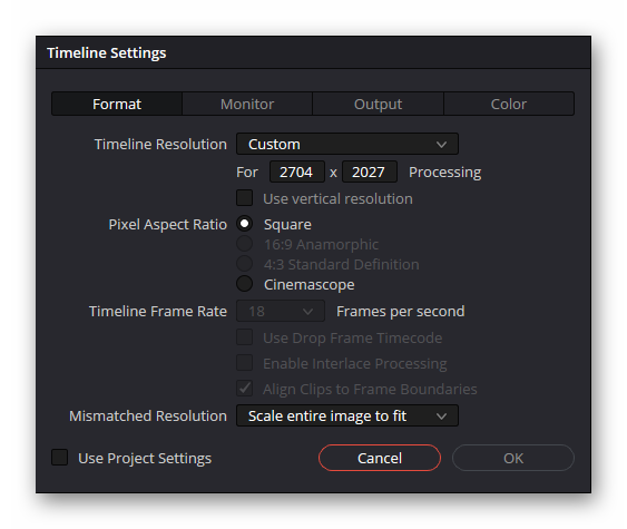
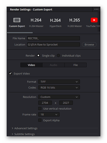
The raw .dng-files from the HQ sensor have a resolution of 4056 x 3040 px. This resolution is reduced, mainly to limit workloads, to an intermediate resolution of 2704 x 2027 px. All processing steps interchange data as such single frames, encoded with rec709, as 16-bit .tif-files.

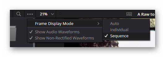
In order for DaVinci to read these separate frames as a complete video, it is important to go to the „Media“ page and make sure that „Media Storage → … → Frame Display Mode → Sequence“ is selected.
grafik
Each frame is large, about 31.3 MB, so a lot of temporary and fast disk space should be available.

Timeline

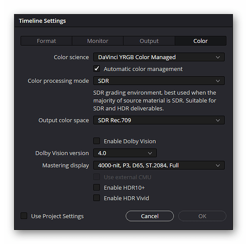
All DaVinci timelines in the following processing scheme share common settings – except the very last one. Resolution is always at 2704 x 2027 px and the fps is set at 18 fps.

grafik

The color science uses „DaVinci YRGB Color Managed“ with the „Automatic color management“ checkbox activated.


In the following, the five processing stages:

  1. Step A: Raw to Sprocket
  2. Step B: Sprocket-Registration
  3. Step C: Color Grading and Stabilization
  4. Step D: Optimizing the Footage
  5. Step E: Increasing Frame Rate and Final Output

will be described in detail.

Step A: Raw to Sprocket

Goals

This step prepares the raw .dng-files from the scanner for further processing. Basically, the raw files are „developed“ and resized to smaller, more managable file sizes.

Additionally, further initial refinements can be done in this step. For example, with my scanner, the camera is slightly rotated with respect to the film gate. Things like this are corrected in this step. Another important parameter to be fixed in this step is the correct overall exposure of the footage, ensuring maximal dynamic range for the following processing stages.

Processing

The raw .dng-files are inserted as continious footage into the timeline.

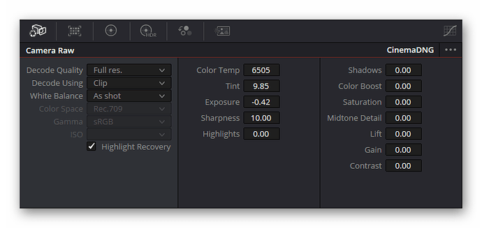
In the „Color“ tab, the settings of the raw reader module have to be adjusted. Specifically, we want the „Decode Quality“ as „Full res.“. Secondly, select in the „Decode Using“ entry decoding on a „Clip“ basis. Only than the various color adjustments available in the raw reader module become active. We will use some of them soon. The „White Balance“ should initally be set to the „As shoot“ mode. Important: do not forget to tick the „Highlight Recovery“ checkbox.

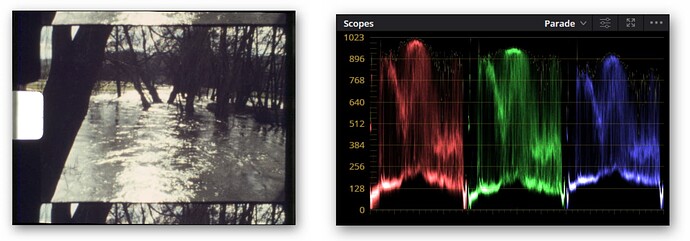
The most important thing which needs to be adapted is the „Exposure“ value of the footage. Find a frame in the footage where some highlights are certainly burned out in the original S8 footage. Normally, it is not difficult to find such frames. Now adjust the „Exposure“ value so that these highlights end up in the „Scopes→Parade“ display just barely below the highest values possible.

Normally, we’re done at that point. Occationally, I tend to adapt the „Color Temp“ in the raw reader module as well as the „Tint“ value here, to push the colors sligthly towards the direction I want them to be.

Adjustments can also be done by switching to the „Primaries – Color Wheels“ or even the „High Dynamic Range – Color Wheels“ tab of the “Color” page. If you footage consists of only a single 15 m S8 roll, that might be an option. You could just do the whole color grading at that step and call it a day.

However, for longer S8 footage, you will encounter issues prohibiting using such a single global color grading/processing run. Here’s a list of things which might interfere with such an approach:

  • Different S8 15m rolls, even when processed by the same lab at the same time, do show different color casts.
  • The original footage scanned might intermix footage of different film brands. Every film stock needs another color science.
  • S8 film/cameras did work only in two modes colorwise: Tungsten and Daylight. So mixed light situations, which were more the rule than the exception, delivered sometimes rather weird orginal colors.

All of the above points suggests to defer the color grading to a later processing stage, where each single scene is graded individually.

Output

As already remarked, the „Deliver“ module of DaVinic is usually set up to output each frame as .tif-file with 16-bit dynamic range. The 16-bit setting is important and ensures that no dynamic is lost.

The above format is actually my prefered format for the whole processing pipeline. One could use the compressed format („Codec : RGB 16 bits (LZW)“), but the uncompressed .tif-format is easier to use with other software.

I generally tend to save all frames in separate directories. So the output of this step is saved in a directory called „A Raw to Sprocket“, with the frame names starting at „REC709_00000000.tif“ and so on.

Step B: Sprocket-Registration

This step, sprocket registration, might not be necessary for some scanner setups. It is however mandatory for my scanner consiting mainly of rather flexible 3D-printed parts.

Furthermore, one could actually handle this task already at the previous step, while in DaVinci Resolve, with appropriate trackers. I prefer to use my own software.

The output of this step ends up in the directory „B Color and Stab“, with file names starting at „SPR_00000000.tif“ and so on.

Step C: Color Grading and Stabilization

The next step is where most of the fun work will be happen. Two major goals will be achieved: first, each scene will be colorgraded individually. Secondly, each scene will have the camera stabilized – this is a major step improving the visual quality of the footage, and a necessary step for the success of the following spatio-temporal degraining/enhancement step.

Color Grading

Color grading is split into two different stages: a fine-tuned global grade, followed by a final individual color grade for each scene.

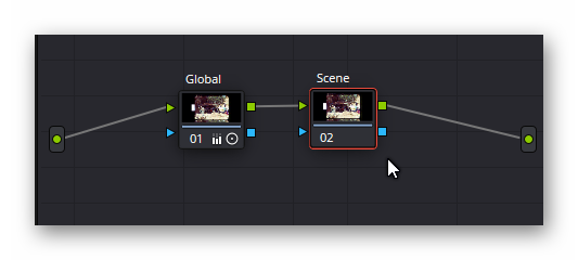
In fact, the global grade could have been applied already at Step A or B in the pipeline. I prefer to do this at this step. Accordingly, the current work flow I am using is based on a two-node structure in the „Color“ page. The first node is used to achieve a good global overall color setting, the second node takes care of individual needs of each scene. There are other posibilities to set this up, I currently prefer the way described in the following.

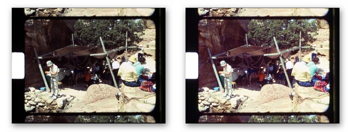
To set up the paramters of global color node, I search for a frame which features ideally the whole range of intensities of the footage. That is, it should feature burned out highlights as well as deep shadows. Great if the scene also contains various gray regions with different intensities. Here’s an example of such a frame (left the original version, right the globally color graded version):

Now check that the burned-out highlights stay below the maximal intensity, by using the „Scopes→ Parade“ viewer. That should be the case, as we have taken care of this already in Step A. Otherwise, adjust the „Gain“ of this global node accordingly.

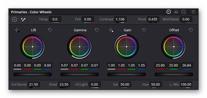
Next thing to check is the „Gamma“ value. Most probably, your image will be too dark, so raise this value a little bit until you are satisfied. While you’re at that, increase the „Shad“(ow) value to push the shadows out of the dark.

The next step is to „get the colors right“. This is kind of difficult and depends also on personal preferences. Here’s my current procedure:

  1. Watching closely the „Scopes → Parade“ viewer, I usually change very carefully the „Offset“ of a single color channel (in my footages, that’s usually the blue channel) so that the colors seems to be more natural.
  2. I adjust slightly „Col Boost“ value. This will increase color saturation of less saturated colors but will leave the highly saturated colors as they are.
  3. Adjust the „Contrast“ value to your taste.

Another option for step 1 above (which gives a slightly different control feeling and result) is to use the „Temp“ and „Tint“ values to achieve a better color reproduction.

You will need to iterate over all of these settings, starting from the „Gamma“ setting. Iterate until you are satisfied. The goal is to get an overall color correction which works ok for all of your footage. Be sure to check that the setting you achieved on your test frame works ok for the other scenes of your footage as well. Always have a careful look at your „Scopes → Parade“ viewer that no clipping of intensity values occurs. In the example above (A Kodachrome frame) I ended up with the following grade:


Your color grading process might differ substantially from this. Have fun!

Once you are satisfied add another secondary node by „ALT-s“. Your clip node graph should look like that:

grafik

This new node will be soon used to color-optimize each individual scene. Note that at this point in time, the whole footage should appear as a single clip in the „Color“ page.

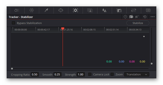
We are in the process of setting up things we want to be identical for all scenes of the footage. Therefore, we go now to the „Tracker – Window“ tab and select in second panel “Stabiliation” the camera stabilization. We want to change two settings here. Deactivate the „Zoom“ checkbox and select in the neighbouring Menu „Translation“ as the basic mode of operation. All other settings can be left at their default values. It should look like this:

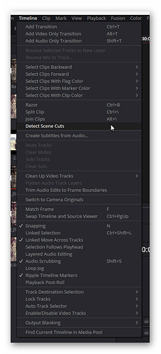
Once that is done, it is time to separate the footage (which is displayed still as a single clip) into separate scenes. You can do this manually, but the automatic scene detection of DaVinci works faster and is usually quite precise. So go to the „Cut“ or „Edit“ page, select with your mouse pointer the whole clip, and than activate the scene detection by selecting „Timeline→ Detect Scene Cuts“.

DaVinci will start to do its work.

Once the scene detection has finished, be sure to check the detected cuts. Occationally, some cuts are not detected, some bad frames will introduce clips consisting of only one or two “flash” frames, and some cuts might be simply wrong. Be sure to correct those bad cuts either in the „Cut“ or „Edit“ page, by deleting the cuts, deleting bad frames or introducing additional cuts where necessary.

Now, since have we set various parameters before we did the split into scenes, every scene will have the global color grading node as well as the default parameters for tracking already set up. That „setting before cutting“ saved us a lot of typing.

Let’s explain the tracking parameters chosen. By deactivating the „Zoom“ checkbox, we prohibt DaVinci from applying any zoom to cover up frame parts with no data. We do need all data for the following processing steps.

The „Translation“ mode of the stabilizer is the most robust tracking mode. And it will reduce the typical amateur camera’s shake considerably.

A little more challenging to compute for DaVinci is the „Similarity“ mode. In addition to the „Translation“ mode, it will also correct rotational movement of the camera. However, in „Similarity“, also zoom is analyzed and corrected – this is not what we want and it tends to screw up the stabilization generally. „Perspective“ is even more demanding and generally not useful for our purposes.

So, once you are satisfied with the scene cuts, select the first clip and go to the tracker in the „Color“ page. Stick for the moment to the „Translation“ mode and analyze each of the scenes in turn. That is, simply click on „Stabilize“. Check the results. Go to the next scene.

Occationally, for certain scenes where the camera moves through a space, „Similarity“ or even „Perspective“ might give you better results – try out these modes, but only if „Translation“ does not yield satisfactory results.

While you’re at a specific scene, use the secondary color node to optimize your color grading to your taste.

I usually create a second grading version by pressing „CTRL-y“. All versions can be displayed via „CTRL-ALT-w“. The currently active grade has a white frame around it. Pressing „CTRL-ALT-w“ again gets us back to normal full screen preview

You can cycle between versions in the full screen view by pressing either „ CTRL-b“ or „ CTRL-n“ (in the „Color“ page, of course). Going to the next scene can be done by pressing „DOWN-arrow“, going back to the previous scene with the „UP-arrow“. Continue to grade and stabilize all scenes of your footage.

Step D: Optimizing the Footage

S8 material can be very grainy; to design great lenses for such a small format is challenging as well. So the visual quality of S8 material is certainly not great.

Since I am more interested in the content of historical footage than the film look of the S8 material itself, I tend to do quite some image processing before the final grade. The goal in Step D is the removal of film grain and the increase of the overall resolution of the footage.

I do this by a combination of various software: a driver program written in Python which creates various configuration files, VirtualDub2 as preview program and avisynth with a bunch of libraries, most noteably a bunch of software routines („TemporalDegrain“) based on the „mvtools v2“-library, doing most of the work.

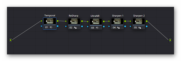
Similar processing can be achieved with the spatio-temporal smoothers available in DaVinci, setting up a node graph like so,


or by using plugins like „Neat Video“ for that purpose.

Side Note: Spatio-Temporal Denoising

The basic idea is quite simple: S8 footage is not sharp for two reasons. One is that itis limited by optics (or physics). The other is of course the film grain. If one trys to increase the sharpness, the film grain is enhanced as well. For improving image definition, we first need to get rid of the film grain, than a very slight sharpening can recover image detail which is otherwise lost in grain.

Now, film grain has a strong spatial correlation. That is, neighbouring pixels „see“ the same colored film patch. They are thus quite similar and this makes it challenging to use spatial noise reduction. However, the temporal correlation of film grain (the difference between consecutive frames) is basically zero – so averaging the same image area over several consecutive frames reduces film grain quite well. That’s why the first node in the above node graph does exactly this: temporal noise reduction. It is followed by a node which slightly resharpens the footage to prepare it for the next node, the spatial noise reduction node; in that node, I am using here the newer (DaVinci v19) „UltraNR“ mode, but other choices are possible. The output of this node is piped into two serial nodes, doing both a slight sharpening. Using two nodes here allows to tune differently sized spatial detail independently from each other.

As one can imagine, there are a lot of parameters to get about right in this process. At this point in time, I decided to implement that processing part via VirtualDub2, combined with avisynth. I came up with five differently parametrized, quite different processing pipelines, for film stock ranging from Kodachrome (very low film grain) to „Revue S8“ film stock (as grainy as can be).

Step E: Increasing Frame Rate and Final Output

In the last step of the processing pipeline, things deviate in the timeline setup. This time the timeline resolution is at only 1440 x 1080 px, that is, HD format. You might opt for other format choices; more important is the framerate setting of this step. In this last step, we work with 30 fps. Color handling is again done via „DaVinci YRGB Color Managed“ with „Automatic color managment“ selected.

The reason is that we want to increase the frame rate of our footage to todays standards. This will lead to a smoother visual experience, especially with fast panning motions. For such motions, the standard 18 fps of S8 material is just too slow. One can easily notice jittery movements of objects and frames in normal S8 footage. Let’s see how this is done once we have created our 30 fps timeline.

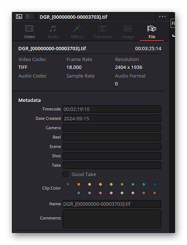
We achieve the retiming by loading the stack of frames from Step D into the timeline. Make sure that it is loaded with 18 fps, by checking the „File“ tab in the „Inspector“:

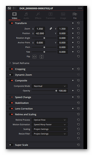
Now it is time to set up the retiming process. This is done in the „Video“ tab of the „Inspector“. Select the following retiming parameters: „Retime→ Retime Process“ is set to „Optical Flow“ and „Retime→Motion Estimation“ is set to „Speed Warp Faster“.

The tab should look like this:

We are using here the same trick as before, that is “setting before cutting” to set further things equal for all clips. So the next thing to do it is to to set an appropriate „Zoom“ value for the footage. With my scanner, a value between 1.2-1.4 gets rid of all border and sprocket areas I do not want to have in the final rendering. Usually, that global zoom value works for most of the footage; occationally, with very strong camera movements, this value migth need a scene-specific modification, sometimes even with changing, key-framed zoom values. That depends on how much work you will put into optimizing a single scene.

We are now in a position to separate the whole footage into separate scenes. This step is absolutely mandatory for the retiming process to work properly. If we fail to do so, the retiming process will create funny transitions between scenes. For cutting the whole footage into different scenes, we go either to the „Cut“ or „Edit“ page, select the whole clip and activate the scene detection by selecting „Timeline→ Detect Scene Cuts“, as done above.

The next step in the process is to go to the „Color“ page and switch from the clip-based node graph to the timeline graph. This graph will be initially empty. „ALT-s“ adds a do-nothing node in this graph. With this node selected, go to the „Blur – Sharpen“ tab of the „Color“ page and select the second entry „Sharpen“. Select a frame with detailed image structure and slowly reduce the „Radius“ from it’s default value 0.5 down towards 0.4. Do not sharpen too much, I usually work with a value of 0.44 -0.47 or so. You can also test various „Scaling“ values. I leave that most of the time at the default value of 0.25, but occationally I raise that a little bit, like towards 0.28 or so. Any node in the timeline node graph will be applied to the whole timeline, that is, to every clip in the timeline. But only after the clip’s node graph has been processed. This behaviour is exactly what we want for the sharpening operation we just set up.

While we’re at the timeline node graph, one can add a second sharpening node and play here again with the „Sharpen“ settings. The goal is to recover fine image details while keeping the sharpening within reasonable limits. Once you are satisfied with the settings, be sure to close the timeline node graph and return to the normal clip node graph.

Finally, it’s time to optimize the grading of every single scene for the last time. Mostly, this will be a little bit of additional color grading, sometimes a new zoom value, sometimes more weird stuff – the possibilities are endless.

Output

We now finally got to the point were we can finally render a real video file. In the „Deliver“ page, I usually select either „H.264 Master“ or „H.265 Master“ and render out. Of course, one could tweek here a lot of settings as well. Check the result before you render out.

7 Likes

Thanks for the elaborate summary of your workflow :grinning:. I recognize a lot of steps from my own workflow, but I’m sure there’s something to take away when I eventually get to editing again.

I’m wondering about the stabilizing process, though. What kind of number exactly is the zoom-setting? Is it a percentage? So far I’ve tried to avoid using it entirely, because I couldn’t determine how much of the image area disappears. From what I understand it’s really a “zoom”, not a “crop”, which means that footage at, say, 2k resolution, gets interpolated in the process. Is there a DaVinci native way to avoid this that I haven’t found yet? I mean, the frame of reference should stay the same across the entire scan, so if “zoom” is actually a percentage, you could set timeline resolution to something like 2k*0.95 and then receive a non-interpolated final video when zoom enlarges it again. :thinking:

Well, the zoom-setting is a checkbox. So you either switch it on or off. I recommend the later.

If that checkbox is checked, a rather complicated algorithm decides what (variable) zoom factor is applied to your footage. You can influence this only a little bit by changing the values in the boxes left to the checkbox (mainly the “Cropping Ratio”). Details can be found in the DaVinci manual. But again, I would not bother; you will have no real control about the zoom factor the algorithm will be choosing. With the checkbox deactived, no zoom at all will be applied; in the case of the “Translation” mode, only pan and tilt compensation.

EDIT: concerning a 1:1 pixel mapping from source to destination - that is difficult to achieve within the context of the stabilization module of DaVinci. It will not be possible at all in the “Perspective” and “Similarity” mode. In these modes, basically not a single pixel in the destination buffer will ever be mapping directly onto a single pixel in the source buffer. The pixels will always end up somewhere between the source pixel positions - which means that interpolation has to happen.

Even in the “Translation” mode, basically it will never happen that pixel positions from source to destination match 1:1 - they will always end up at subpixel positions, necessating again interpolation.

Overall, it’s even more complicated. DaVinci has the concept of a timeline resolution, and this is the resolution all processing nodes use. That is typically different from the source resolution of your media. Again, interpolation is taking place here, already at the input stage. Try to play around with a certain clip by open the “Inspector” tab and change the entries in “Retime and Scaling → Scaling” and "Retime and Scaling → “Resize Filter”. Then see what different timeline resolutions do. It might initially be a little confusing…

I’d say that considerations like this do not matter really with S8 material. Most of the material I have delivers something between SD and HD resolution in reality.

Yeah, I just realized I confused Zoom with the Cropping Ratio slider, which for some reason is “higher=less crop” and sadly has nothing to do with percentages.

I also would’ve expected “Translation” mode to just move the image around without altering its dimensions, so it seems strange to me that even then interpolation happens. Or does that only apply if timeline resolution is different from source resolution? So far I’ve only worked in timeline=source resolution as my source resolution was rather low, which also means that the settings under Resize Filter do absolutely nothing :slight_smile:. (But that’s a good hint, anyway. Missed that setting entirely).

Well, let me try to go a little bit into more detail here. But: DaVinci is a closed-source program; that is, my arguments are not based on the actual code – so the following might not be spot on.

Nevertheless, certain image operations can never be done via a 1:1 pixel mapping, and camera stabilization is certain one of them. The reason is rather simple. If a camera moves, say a tiny dot on a white screen might fall at frame N exactly onto a single pixel of the camera. However, nearly certainly, in frame N+1, the tiny spot will fall between two neighbouring pixels. That is the reason (good) stabilizers work with subpixel precision. The shift values calculated from frame NN+1 might be pan = 13.23and tilt = 24.56. Of course, you could just map using only the integer parts, that is, something like pan = 13 and tilt = 25, but that would be imprecise. Higher level stabilizers (and I am sure DaVinci’s stabilizer is of that sort) would of course map using the real values. Otherwise, you would notice a small jitter in fine structures.

So: no, even the “Translation” mode of the stabilizer does not give you a 1:1 pixel mapping. You will nearly always end up in sampling between pixels, that is, at subpixel positions. For a lot of things you need that subpixel mapping/sampling and that’s what is done. (Just a side note: mathematically, there is no drawback here; your original pixel values represent in reality a continuous function in a well-defined function space. Resampling that function on intermediate pixel coordinates does not change the continuous function itself, only the discrete (pixel-based) representation of this function.)

Be aware that most likely, other functions available in the “Color” page of DaVinci are also violating your desired 1:1 pixel mapping. Think of rotation, for example. If you are using the “Mid/Detail” control of the “Primaries - Color Wheels” tab, information from neighbouring pixels are used to come up with a new intensity of the central pixel. The “Blur - Sharpen” unit also needs to use information from neighbouring pixels.

There are some functions (so-called point operations) that do use only the intensity of a single pixel. Examples are “Lift”, “Gamma”, “Gain” and “Offset” in the “Primaries - Color Wheels” tab.

Personally, I never bother with these details of the processing pipeline. There will practically be no noticable image deterioration within normal use of DaVinci’s functionality.

2 Likes