Alpha-Release of new picamera-lib: "picamera2" ... - and beyond

Recently, the Raspberry Pi foundation released an offical alpha-release of a new python library, “picamera2” (alpha = things might still change). There are quite a few film scanner approaches using the HQ camera of the foundation in combination with the old “picamera” library. This old library was based on what was available at that time, namely the propriatary Broadcom-stack. This library hasn’t seen any update since about two years.

The new “picamera2”-library is using the new open-source “libcamera”-stack instead of the Broadcom-stack. It is also an offical library supported by the Raspberry foundation. I will report in the following a few insights for people considering to upgrade their software to the new library.

As the “picamera2”-library is based on the “libcamera”-approach, there now exists a tuning file for several sensors, including the v1/v2 and HQ camera of the Raspberry foundation. In principle, this tuning file allows for fine-tuning of the camera characteristics for the task at hand. Because “libcamera” handles things quite differently from the old “Broadcom”-stack, the python interface is also based on a totally different philosophy.

Accessing the camera with the new software is simple, as a lot of functionality is taken care of behind the scenes. Here’s an example taken directly from the “example”-folder of the new libraries github:

#!/usr/bin/python3
import time

from picamera2.encoders import JpegEncoder
from picamera2 import Picamera2


picam2 = Picamera2()
video_config = picam2.video_configuration(main={"size": (1920, 1080)})
picam2.configure(video_config)

picam2.start_preview()
encoder = JpegEncoder(q=70)

picam2.start_recording(encoder, 'test.mjpeg')
time.sleep(10)
picam2.stop_recording()

After the necessary imports, the camera is created and initialzed. Once that is done, a preview is started (which in this case also silently creates a loop capturing frames from the camera). After this, an encoder (in this case a jpeg-encoder set to a quality level of 70) is created and appended to the the image path (picam2.start_recording(encoder, 'test.mjpeg')). The camera is left running and encoding to the file ‘test.mjpeg’ in the background for 10 seconds, after which the recording is stopped.

For a film scanning application, one probably wants to work closer to the hardware. Central to libcamera’s approach are requests. Once the camera has been started, you can get the current image of the camera by something like:

request = picam2.capture_request()
array  = request.make_array('main')
metadata = request.get_metadata()
request.release()

From aquiring the request until you release it, the data belongs to you. You have to hand it back by request.release() to make it available again for libcamera.

Besides the image data (which you can get as numpy-array (request.make_array('main')) as well as a few other formats) every request has also a lot of metadata related to the current image. This metadata is bascially a dictonary which is retrieved by the request.get_metadata()-line. Libcamera operates with three different camera streams, one of them is ‘main’ (which was used in the above example). These streams feature several different output formats. One called ‘lores’ operates only in YUV420, another one called ‘raw’ delivers just that: the raw sensor data.

Some (but not all) of the data returned in the metadata dictionary can not only be read, but also set. For example, the property AnalogueGain is available in the metadata - this is usually the gain the AGC has selected for you. It can also be set to a desired value by using the command:

picam2.set_controls({'AnalogueGain':1.0})

One notable example of a property which can not be set is the digital gain. More about that later.

Some properties of the camera can also not be set in the way described above, mainly because they are related to requiring a reconfiguration of the sensor. One example is switching on the vertical image flip, which can only be done in the inital configuration step, like so:

video_config["transform"] = libcamera.Transform(hflip=0, vflip=1)
picam2.configure(video_config)

Another important deviation from the old picamera-lib is the handling of digital and analog gain. In the new picamera2-lib, there is actually no way to set digital gain. As the maintainer of the library explained to me, a requested exposure time is realized internally by choosing an exposure time close to the value requested and an appropriate multiplicator to give the user an approximation of the exposure time requested.

An exposure time of, say, 2456 is not realizable with the HQ sensor hardware. The closest exposure time available (due to hardware constraints) is 2400. So the requested exposure would be realized in libcamera/picamera2 by selecting: (digital gain = 1.0233) * (exposure time = 2400) = (approx. exposure time = 2456).

This behaviour spoils a little bit serious HDR-work, as the data from the sensor is only an approximation of what you actually requested. And there exist differences between frames taken for example with exposure time = 2400/ digital gain=2 (a combination the AGC will give you occasionaly when requesting exposure time = 4800) and exposure time = 4800/ digital gain = 1.0 (which is the actual desired setting).

One approach to circumvent this is to choose exposure times which are realizable hardware-wise and request this exposure time repeatably (thanks go to the maintainer of the new picamera2-lib for this suggestion), until the digital gain has settled to 1.0. For example, the sequence 2400, 4800, 9600, etc. should give you in the end a digital gain = 1.0. And usually, it takes between 2 and 5 frames to obtain the desired exposure value.

By the way, the old picamera-lib had a similar issue. With the old lib it took sometimes several frames until the exposure time settled to the requested value.

I am currently experimenting with a few approaches to circumvent this challenge. Based on a suggestion from the maintainer of the library, namely to request a single exposure time until it is delivered, before switching to the next one gets me a new exposure value every 5 frames on average.

With this approach, my current scan speed is about 3 secs per movie frame (2016x1502 px). This includes taking five different exposures and a waiting period of 0.5 sec to settle out mechanical vibrations of the scanner. Not too bad.

As the maintainer of the library indicated, some work might be done to improve the performance of the library with respect to sudden (and large) changes of exposure values - however, as this might require to change things in the library picamera2 is based upon(libcamera), it might take some time.

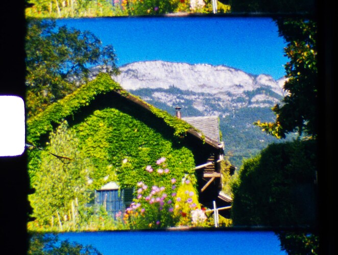
Finally, here’s a comparision of the color differences with the old and new library. The old picamera-lib/Broadcom-stack delivered for example the following frame:

The new picamera2-lib/libcamera-stack gets the following result from the same frame:

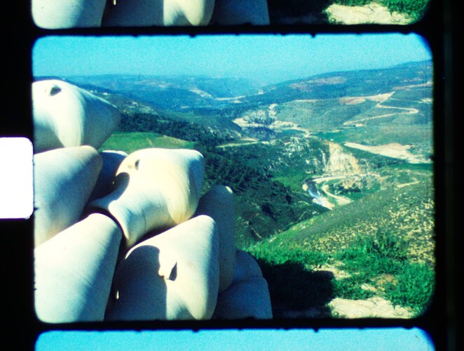
This capture is from Kodachrome film stock. Here’s another capture from Agfa Moviechrome material with the old picamera/Broadcom-stack combination

and this is the result of the same frame, captured with the new picamera2/libcamera-stack:

Two things are immediately noticable: the new picamera2 delivers images which have a better color definition. The yellow range of colors is actually more prominent, which should help the rendering of skin tones. Overall, the new picamera2-lib/libcamera-stack features a stronger saturation, which creates more intense colors. Also, it seems that the image definition in the shadows is improved.

One last note: JPEG/MJPEG encoding is currently done in software, with the simplejpeg-library. So the quality settings of the old library, which used hardware encoding, are not directly transferable. Also, a higher system load is experienced, especially if using the available multiple thread encoder

4 Likes

I also made some tests of Picamera2. Here are some remarks.

The API is quite high level but closely reflects the libcamera API, a bit complicated though. One may regret the simplicity of the original Picamera.

You should not expect any better performance at all and even the opposite.

With Picamera jpeg capture on video port I measure 3fps in full resolution 4056x3040 and 13fps in binned mode 2028x1520.

With Picamera2 the loop on request without copy of the numpy array nor encoding gives 30fps in binned and 9fps in full, the library can practically follow the fps of the sensor, it’s good. But if we get the numpy array and encode it to jpeg we fall to 5fps in binned and 1fps in full mode. On the other hand the possibility to have the metadata without the full frame is interesting.

I don’t really agree with your explanations on the digital gain. It is not a problem of AGC because when setting the exposure we stay in AeEnable = false nor a problem of realizable exposure

Here is a sequence of requests that starts from exposure 571 and that we ask 6514 with AeEnable = false
AeLocked: False Exposure: 571 Analog: 1.0 Digital: 4.0
AeLocked: False Exposure: 6485 Analog: 1.0 Digital: 1.0043612718582153

The value 4 for the DigitalGain is strange. I think that as you ask for an image with exposure 6514 and the library receives from the sensor images with exposure 571 it thinks it is useful to you by applying a digital gain! These frames must be ignored. Then 6514 is not feasible so we stay at 6485 with a digital gain of 1.004, it does not seem really annoying. It seems moreover that this behavior appears only in the increase of the exposure case.

There are two things which push me towards the new library. For one thing, let’s face it: it’s the future. The old picamera-library has not seen an update in two years, and any new Raspberry Pi stuff will be based on the new libcamera-approach. Second, and actually more important for me: the color definition has certainly improved with the new approach (as one can see from the images above).

One current big drawback, especially if you transfer jpeg-compressed images via LAN, is that jpeg-encoding is done in software. With the old Broadcom/picamera combination, this was utilizing a hardware module. With the libcamera/picamera2 combination, it is pure software-based for now. There exists a framework in the picamera2 code which allows multiple encoding threads which will speed up things a little. The drawback is that the system load gets easily close to 100% with 4 encoding threads.

Nevertheless, I do see in my usual client/server setup (server: RP4 with HQ cam, images encoded as jpeg/client: WIN10-PC, Intel Core I7-87000 @ 3.20 GHz) a frame rate of 6.7 fps at a quality level of q=95, and a frame rate of 8.3 fps for a quality level q=60. These numbers are obtained with a sysload of about 26% of the RP4. The HQ sensor is running in these experiments at 4056x3040 px (i.e., not the binned mode), with libcamera scaling down the image to a 2016x1520 resolution (this is the jpeg transferred via LAN to the WIN10-PC). Jpeg-encoding and transfer of the image via LAN is currently done directly in the capture thread, not in separate threads. So there is the possibility that these numbers can be improved. Not so bad for the moment.

The secret to run the HQ camera with highest resolution (mode=3 in the old syntax) but get a non-binned scaled down version of the capture is the following initialization sequence:

picam2 = Picamera2()
video_config = picam2.video_configuration(main={"size": (2028,1520)}, raw={"size": picam2.sensor_resolution})
video_config['main']['format']= 'RGB888'
picam2.configure(video_config)

The second line is the important one: the part raw={"size": picam2.sensor_resolution} switches the sensor to the old mode3 (full sensor resolution, max 10 fps). The “main”-profile (the one which is later used for scanning) is requested by main={"size": (2028,1520)} to be of a size of 2028x1520. Now, picamera2 defaults to image sizes quantitized in x-dimension to 16, for speed reasons. So it will actually silently reconfigure the output to a 2016x1520 px size. Finally, a little further speedup can be achieved by asking the pipeline to drop the alpha-plane by requesting video_config['main']['format']= 'RGB888' for the main profile.

Well, that was what I observed and what the maintainer of the picamera2-lib explained to me. To put it simple: digital gain is gone. There is no way to set it to a desired value within the context of the picamera2-lib.

The reason is the following: as I tried to explain above, not every exposure time can be realized by a given rolling-shutter sensor. Exposure times have to be multiples of the time it takes to scan and transfer a single sensor line. So what to do if a user requests an exposure time of 2456 which is not realizable by the hardware?

Well, the trick is simple: choose an exposure time you can realize with the sensor in question (in the case of the HQ sensor that would be 2400) and make the missing exposure up by ramping up a little bit the digital gain from the default value of 1.0. So if you ask for exposure time = 2456, in reality the sensor will work with exposure time = 2400 and a digital gain = 1.0233:

2400 * 1.0233 = 2456

That is the reason why with the libcamera/picamera2 combo, digital gain is gone. You still can set the analog gain, you still can set the exposure time. But every time the requested exposure time is not compatible with the hardware, you will end up with a digital gain slightly above 1.0.

Now, there is even an additional twist. Let’s assume you ask for an exposure time of 2400 - which can be realized exactly with the HQ sensor.

Now, in order to give you the requested exposure as fast as possible, libcamera might opt to select for a few frames not the desired 2400*1.0-combo, but work instead with 1200*2.0 or even 600*4.0. All these products of (hardware) exposure time times digital gain give you the same, namely 2400.

I must say that in principle this idea of using the digital gain for approximating arbitrary exposure values within the constraints of the hardware is basically not bad. However, the game is spoiled for serious HDR-work, as the images with the above “alternative” realisations do look different from each other.

Anyway, with that understanding what is going on with the digital gain in the new libcamera-lib, the numbers you have cited above from your experiments make perfectly sense to me. For example, the digital gain = 1.0043612718582153 simply indicates that an exposure time of 6485 is not realizable with your hardware.

The maintainer of the picamera2-lib knows about this issue and he promised me to look into this. As it might require changes in libcamera itself, it might take a while.

By the way, from my experiments, it takes about 11 frames until an exposure change has propagated through the picamera2/libcamera pipeline and shows up in the metadata of the current exposure. Even if you asking for exposure values which can be directly realized in hardware, you need to at least request the same exposure value 5 times in a row to reliably obtain the requested exposure time with digital gain = 1.0. Some details can be found here.

2 Likes

Some further insights into the new picamera2/libcamera-approach. The guys developing this do all kinds of fancy stuff - which might be nice for the average user, but troublesome for our purposes. However, as the new approach is more open-minded, you have more influence about the outcome of the whole process.

Let me give you an example. The new libcamera-stack includes something which is called (alsc). This is the short for “Automatic Lens Shading Correction”. These algorithms can be user-tuned with an own tuning file, but by default a tuning file is used which is shipped with the libcamera installation for various sensors.

Now, lens shading is usually used to compensate for deficiancies with a certain lens/sensor combination. Most interestingly, the tuning file for the HQ camera, which is not delivered with specific lens, includes a alsc-section as well! I have no idea what lens was used here during calibration, but certainly it is not the lens I am using in my scanner setup.

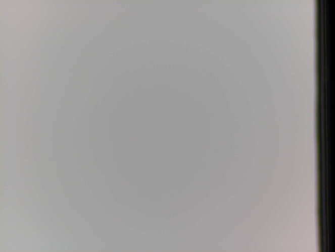
Any indeed, if I look closely at a capture of the empty film gate (I have reduced the q-parameter of the image to utilize banding to show better the issue),

you see that the image center is darker than the image egdes. Also noticable is an annoying pink cast, especially in the right image corners.

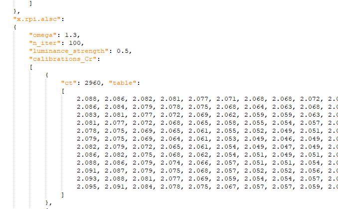
Continuing our little experiment, I disabled the alsc in the tuning file - which is simple enough, you only need to change the original rpi.alsc on line 207 of the original tuning file to x.rpi.alsc, like shown in the following screen shot:

Screenshot 2022-06-18 100201

After this little surgery I get a much improved flat response:

EDIT (28/06/22): originally, I gave below an example that the colors of an image changed drastically when switching off the ALSC. I am not so sure any longer that this was the real reason. It seems that the new libcamera-stack behaves somewhat arbitrary when you set the red and blue gains - the AWB-algorithm than spits out a somewhat arbitrary color temperature which is in turn used for selecting the ccm-matrices which take you from camera RGB to sRGB. This might be the main effect for the change in color appearance reported below.

I’ll leave the original post below, just in italics.

The bad thing about this is that the color boost observed between the old picamera/Broadcom combination and the picamera2/libcamera compo is gone as well. Here’s a quick example of a scan with the alsc

and one with the alsc turned off:

That looks very similar to results obtained with the old picamera/Broadcom combo. So it seems that the adaptive lens shading is doing more than lens shading correction only. Oh well…

Clearly, it would be perfect if one could come up with an optimized tuning file for film scanning. Theoretically, one could do such a calibration; there is tuning software available. However, this tuning software requires you to take a series of images, flat and with specific color-checkers imaged. At the moment, I have no idea how to do this (specifically: getting the color-checker into the small Super-8 frame for imaging). Any ideas are welcome!

2 Likes

Thank you for sharing these insights. Working with the camera is on my list, and having these postings would certainly save me a great deal of time, since I am hoping to use the new library.

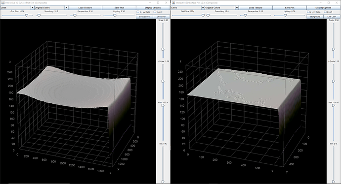
In this article about the Universidad de la República updates of their scanner, they listed an interesting plug-in for creating surface plots from an image for 3D visualization. I have not used any of it, but a similar graphical representation would be a great way to illustrate the alsc issue.

PS. here is a quick comparison of the images above from @cpixip which enhances the visualization of the alsc unintended consequences for film scanning.

This is an excellent tool to visualize and evaluate the flatness of the scanner components chain (light+lens+camera).

2 Likes

Here’s a current update of my research into the new library/python-combo libcamera/picamer2:

  • as with the old Broadcom/picamera pipeline, the new combo is geared towards the goal “create a nice picture out of what you are seeing”. This is quite contrary to the goal of a camera for scanning film stock. Here, you want constant imaging parameters from frame to frame - you do not want to introduce image variations by changing camera parameters.

  • it was hard to achieve that goal with the Broadcom/picamera combo, but, at this point in time, it seems close to be impossible with the libcamera/picamera2-stack. The reason is an attempt to be user-friendly (=more automatic stuff you cant turn off) and make cheap hardware look nice (=more image processing algorithms thrown into the equation).

  • An example might be the lens shading algorithm discussed above. Lens shading was already available in the old Broadcom/picamera combo, consisting of just a single matrix for the R-, G- and B-channels. With certain variants of the picamera-lib, it could be directly set in the user’s python code, even during the camera delivering frames. In the new libcamera/picamera2 combo, lens shading is deferred to the tuning file, so it is no longer possible to change it on the fly.

  • even worse, the camera calibration tool writes different lens shading tables for varying color temperatures into the tuning file. This is of interest in the context of mobile phone cameras and the like. Mainly due to low-cost IR-filters used here, specifically the lens shading of the red channel changes noticeably when the color temperature (ct) changes for example from 2400 K to 6400 K. Of course this is not really an issue with higher quality components.

  • the current color temperature is estimated within the new approach by a libcamera-module which is not too precise. It fails in a big way if the illumination is not similar to a black-body radiator (that would be something similar to a incandescent lamp). An illuminated sphere with a three R-, G-, and B- LEDs is very far from a black-body radiator. So this is an example where the ct is estimated wrong. The possibly incorrect ct is used in turn by the ALSC-algorithm to select an appropriate lens compensation table - not a good situation within a film scanning environment. Here are visualizations of two of the lens shading tables for the IMX477 at different cts (while the variation is modest, it is certainly nothing you want to have while scanning film.):

  • the other trouble hiding in the ALSC-algorithm is the “A”, which stands either for “automatic” or “adaptive”. There is actually an adaptive algorithm running in the background which modifies the static lens shading tables, lastly applying a lens shading compensation which is somehow adapted to the scene the camera is viewing. In reality, the ALSC computes local multipliers for each of the color channels, trying to align neighboring image patches to “look the same”. Probably not a thing you want to do if you are trying to scan film faithfully. At this point in time, I am not aware if there is any possibility to switch off this adaptive behavior. So you are left with only one choice: switch off the ALSC completely (as described above). There seems to be no possibility to use static and predefined lens shading tables, for example to counter an unevenly illuminated film window. That was possible in the old Broadcom/picamera combination.

Finishing off today with the following remark: the available documentation for libcamera and specifically the Raspberry Pi version is horrible. Most of the time you need to analyze directly the available source code to get some idea how things are done. It’s even difficult to locate the relevant source code files and: some important parts are not available at all (specifically: the real implementation of the Raspberry Pi’s image processing pipeline. Only the code of the control algorithms for the pipeline seem to be available).

So, all in all, while the Raspberry Pi environment might potentially be a nice and affordable camera platform for film scanning (and other, more scientific uses as well), the current software interface (mainly libcamera) is ill-designed, mostly undocumented and challenging to use. I am afraid this will be a showstopper for any slightly professional application.

4 Likes

… continueing my journey into the unknown. Picking up this remark of mine:

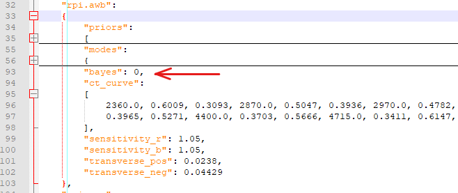
Well, there is a way to get the AWB algorithm starting to work with RGB-LEDs. If you change in the tuning file for the HQ sensor, “imx477.json”, the entry rpi.awb-bayes from the value “1” to the value “0”, like show in the following screen grab,

grafik

the AWB seems to be working again (see below for details). If so, the reported ct is fixed to 4500 K. Which in turn fixes also the ccm-matrix. The one reported by the camera,

ccm = [2.01, -0.90, -0.11, -0.38, 1.82, -0.43, -0.10, -0.57, 1.66]

is slightly different from the closest ccm given in the tuning file (ct = 4400 K):

ccm = [2.0, -0.95007, -0.10723, -0.41712, 1.78606, -0.36894, -0.11899, -0.55727, 1.67626]

This is probably due to the CCM-algorithm interpolating for the “estimated” ct of 4500 K between the two ccms given in the tuning file closest to this value, namely ct = 4400 K and ct = 4715 K.

Details: the AWB tries to estimate the current color temperature based on some heuristics. For example, these heuristics are a tendency toward cooler illuminations if the illumination is bright (there’s a module in the libcamera-pipeline to estimate a lux-level for that purpose), and toward warmer color temperatures if the estimated illumination levels are low (candle light would be an example). In certain cases, the build-in heuristics fail. One case is the RGB-LED light source discussed above, another case I know of occurs if the IR-filter in front of the sensor is removed. For such cases, there exists a simple algorithm, termed “Grey World”, which only tries to make the full image “grey” on the average. It is the default when "bayes": 0 is selected. It works actually rather well, provided your image does not feature a prominent red (sun set) or green (dense forest) or blue (underwater photography) cast. Lastly, "bayes": 1 is the default setting in the tuning file, named this way as the algorithm then uses Bayes’ Theorem for the estimation of color temperature.

2 Likes

What would be the negative effect by turning off ALSC in regards to the lens shading that then can’t be accessed? Is the result chromatic abbreviations in the resulting image?

Short answer: no.

Short answer: I could not detect any visible disadvantage of turning that thing off. (But please read on if you want to understand the whole story.)

Longer answer(s): Simple lenses have strong chromatic aberrations. Without going into much detail, chromatic aberrations manifest themself mainly in color fringes seen around strong contrast edges in the image.

For the last century, reducing these type of lens errors has been one of the holy grails of the optical industry. It is partly science and partly an art to do this, requiring the careful combination of different lenses made out of different optical glass.

Recent advances in processing speed and power have made it possible to somewhat reduce the color fringes of simple lenses by appropriate computations. This enables you to use cheaper designed lenses. Therefore, this trend is mainly followed in mobile phones and cheap cameras. A good (and therefore quite expensive) prime lens does not need such a computational correction.

In any case, the ALSC has nothing to do with chromatic aberrations. It has something to do with another challenge in optical design (and there again with the drive to solve this cheaply for economic reasons). The design challenge in question is called “vignetting”, and it can again be seen most prominently in cheaply designed lenses. Here’s an example taken out of the Raspberry Pi tuning guide:

grafik

The left image shows the image as it is originally recorded by a specific lens/HQ camera combination. The image is clearly darker around the edges than in the center of the image. Traditionally, this used to be compensated via a lens shading algorithm correcting the luminance appropriately. The outcome of this can be seen above in the center image. This looks better. But, looking closely and you should discover a greenish tint still present around the egdes of the image.

This greenish tint is also the result of an economic optimization - it is mainly caused by the IR-blocking filter of the sensor and small sensor sizes of current camera designs (here’s more detail). In order to get rid of this tint, different lens shading tables for each color channel and - more importantly - for different illuminantions (color temperatures) are needed. If done correctly, one gets the right image displayed above out of the camera instead the middle one. That is the purpose of the ALSC.

So why am I discussing above turning off this image perfecting algorithm?

Well, there are several reasons:

  • First of all, you might not need this. In my use case (a good large format lens) I do not have any luminance vignetting. Furthermore, since in my setup the distances between lens and sensor/movie frame are large, the optical rays are nearly parallel to the optical axis. Combined with the replacement of the stock IR-blocking filter I do not have chromatic vignetting either. So in a way, the camera outputs directly the image above on the right.

  • Second, the algorithm is poorly described. I really tried hard to gain insight into this thing, even trying to locate the source code. The most detailed account I found was in the “Raspberry Pi Camera Algorithm and Tuning Guide” in section 5.9.3. But frankly, that is not a very satisfactory explanation of how the algorithm works. I think it applies some sort of local color balancing, but that assessment is wild guesswork at best. Definitely the algorithm runs only sparesly, its effect is not updated on every image delivered by the camera.

  • the color part of the ALSC algorithm relies on an exactly calculated color temperature and this information might not be available. For one thing, color temperature is estimated by yet another algorithm, namely the auto-whitebalancing. Estimation of the color temperature is no easy task, especially when dealing with LED-based illumination, so it can fail. In this case, the wrong lens-shading tables would be applied by the ALSC. The same happens when you have switched off the auto-whitebalance algorithm, for example by setting one of the red or blue gains. Of course, all of this is undocumented so far.

  • Lens shading tables are only valid for a specific lens/sensor combination. So it’s quite amazing that the HQ camera is supported by the Raspberry foundation with a tuning file including lens shading information for three different color temperatures. Remember: the HQ camera is shipped without a lens - you need to select and purchase one on your own. I actually asked the foundations engineer what lens data was included in the tuning file and got only a somewhat vague answer:

therealdavidp wrote:

Mon Jun 20, 2022 8:19 am

… the supplied tuning is indeed a fairly “generic” tuning that works reasonably well with both of Raspberry Pi’s recommended lenses.

[cpixip] wrote:
That’s what I thought. You probably used the 16mm 10 MP Telephoto lens for the calibration?

Possibly, too long ago!

So, finally coming back again to your question:

It will depend on the lens you are using. If your lens exhibits vignetting, you probably want at least the luminance part of the ALSC running. But: you need to create the appropriate lens shading tables for your sensor/lens combination, you can not use the ones supplied by the Raspberry foundation. If your lens/sensor combination in addition exhibits color fringes, you will need to run through the whole calibration procedure described in the camera tuning file (linked above).

As it is rather simple to activate and deactivate parts or all of the ALSC via tuning file editing, I recommend at this point in time to do some experiments similar to the ones I described above with your specific setup/lens. In my case the results were rather clear:

  • running the ALSC with the default tuning file leads to vigenetting and color tints around the edges of the image, as described above.

  • running the ALSC, but with lens shading tables all set to 1.0, is visually identical to not running the ALSC at all. Note however that in this case the ALSC algorithm should do something (current guess: locally adapt color balance). But it is not noticable.

  • switching completely off the ALSC. This gives me the best image.

You might come to other results. Depends on the lens.

1 Like

As always, much thanks @cpixip for the deep insight. It is of enormous help now that I’ve started the software part of my project. The idea in one of the Github threads you were in, where requesting the exposure values many times in a row until all frames were grabbed is something I’ll be using in my HDR-approach.

Two questions that springs to mind:

  1. What’s your method of selecting the right exposures for getting the mids, lows and highs in the image. Since that is dependent on the brightness of the lightsource, how do you pick out the specific exposure numbers?

  2. My coding is done on a Raspberry 3B with 1 GB of RAM. I get the camera working normal but when I try to capture in the raw sensor resolution that you showed a bit up in this thread my program crashes due to memory restrains, from what I can tell. How much memory usage do you get on your RP4. I’m thinking if i should get the RP4 4GB, 8 GB or continue searching for a bug that causes the crash.

Hi @Ljuslykta - I assume that you want to go the multiple exposures merged into a pseudo-HDR via the Mertens exposure fusion algorithm. So, on this basis:

Before talking about exposure times, let us consider two effects which change with respect to the difference between neighboring exposures.

  • if you increase the difference between neighboring exposures, you can cover a wider dynamic range when exposure-fusing the images. The maximum possible difference between exposures is given by the dynamic range a single of images can cover. That would be anything between 3 to 5 EVs. Taking exposures further apart will lead to weird merged images.
  • if you decrease the difference between neighboring exposures, the increased image overlap will result (with appropriate merge parameters) in noticeably reduced noise in your scan. This is due to the implied averaging between images happening during exposure fusion.

Next point: the dynamic range of color-reversal film is huge and you probably want to cover most of this range. To do so, you have (again) two options:

  • simply take more than three images for mids, low and high. Each additional image will eat a lot of time during scanning, but it will also decrease the camera noise in your final images. I personally work with 5 evenly placed different exposures I usually name ‘highlight’, ‘prime’, ‘shadow1’,‘shadow2’ and ‘shadow3’. The names are indicating their purpose; other people do fine with only two exposures.

  • increase the difference between two neighboring exposures. You probably can go up to 3-4 EVs, depending slightly on the dynamic range of your camera. My spacing is currently set at 1 EV. That is, the exposure times I am using are given by the following code:

    #### exposure sequence
    baseExposure  = 2400
    exposures     = [  baseExposure*2**4,
                       baseExposure*2**3,
                       baseExposure*2**2,
                       baseExposure*2**1,
                       baseExposure*2**0  ]

Remember, I am working (at the moment) with 5 exposures. If you would use less, you would increase the EV-spacing.

In scanning color-reversal film, you need to take care that the capture with the shortest exposure time (the “baseExposure” in the code above) is short enough not to clip any highlight. In fact, you want to have the highlights of your film within the range where your camera is still working sort of linear. So my baseExposure is selected in such a way that a scan of the empty film gate gets me intensity values of around 240 (from 255 which would be the maximum). Any highlight in the actually scanning film will be less than this, so you can have fun in the post.

Summarizing: the darkest exposure of a stack of images for exposure fusion should be selected in such a way that the pure light source of your scanner is at pixel values of about 240. This fixes base exposure. Than you can play around with the number of exposures and the EV-difference between them to get the result you want.

It certainly will. The switch from the old Broadcom-stack to libcamera changed things. In the old days, you would increase the GPU’s memory size to handle the camera’s ISP running on the GPU. These days are gone. Just leave the GPU memory split on its default. Libcamera uses and needs a great chunk of continuous memory called CMA, and it allocates a default size, depending on the processor. So a RP3 gets not enough of that memory to handle full-sized images, while a RP4 with more memory does.

Try the following: set the GPU’s memory to the default or lower. That should give you a larger chunk of memory for other applications. Include or modify in the config.txt the following line:

dtoverlay=vc4-kms-v3d,cma=512

and reboot. This will set the amount of CMA to the RP4 default value. In case of my RP3, this worked. Your mileage might vary and depend on your other memory needs. In my case, the RP3 is running headless with the VNC-server switched on and only a camera-server active.

If that does not help, you could try to decrease the number of buffers which are allocated by the default picamera2 lib. That number seems to change during revisions of the lib, but it is low, one or two buffers, for still configurations and high, about four buffers, for video configurations. Of course, playing around with these numbers invite libcamera to run out of buffers if you are not careful. I would first try to increase CMA-memory as suggested above.

2 Likes

… continuing my journey into the new libcamera/picamer2 environment. The current “next” branch of the picamera2 lib features the possibility to directly capture raw images in .dng-format (with a qt-based app).

The results I get are however slightly underwhelming.

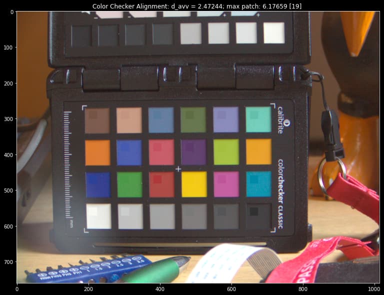
Here’s the result I get when imaging a color checker, using rawpy to read the .dng-image:

The little squares inserted for analysis show how the colors of the color checker’s patches should actually look like.

Clearly, there are some deviations. Especially the blue region of colors seem to be too saturated. I checked the image also in darktable, with the embedded camera matrix as input profile. The result in terms of colors is practical identical.

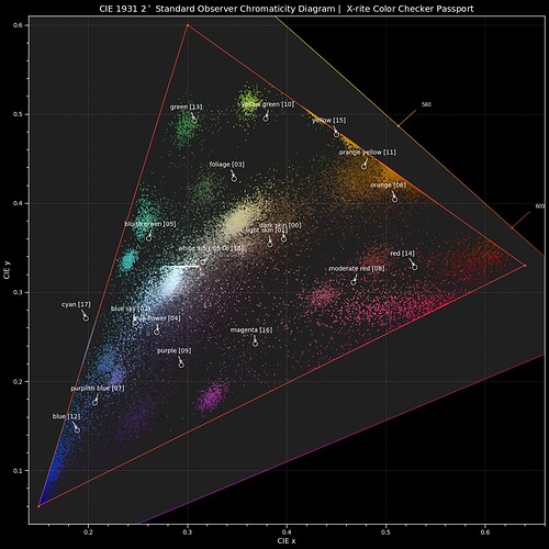
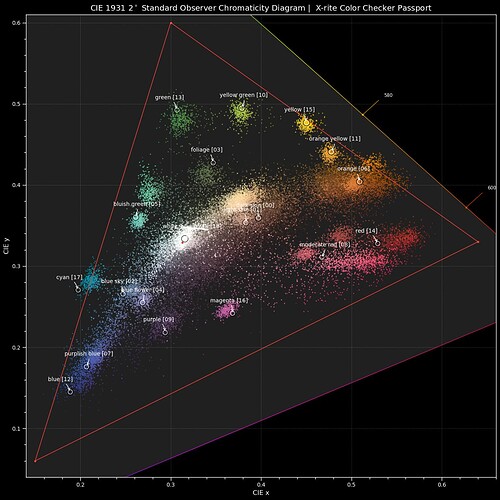
Looking at the CIE1931 diagram, where the real color positions of the color checker’s patches are indicated by little white circles,

one sees again that the imaged colors of the patches are way off. In fact, most are shifted towards the blue, suggesting an error in the estimation of the color temperature (the image was taken with daylight illumination).

At the moment it is unclear to me where the embedded color matrix is coming from (I guess it’s libcamera’s matrix calculated with the data in the tuning file), but it seems that this color matrix is not spot-on. I am still investigating this issue.

However, for demonstration: you can do better. Here is the result obtained from the raw file data with another color matrix:

The color matrix used in the above display was calculated in such a way as to maximize the similarity between real patch colors and image colors.

There are still noticeable deviations, but much less so. Here’s the CIE1931 diagram of this image

showing a much closer approximation of the true colors of the patches.

So the HQ sensor is able to closely reproduce the real colors of a scene.

I have not checked yet whether the above performance also applies if not raw but normal jpeg-images are output by libcamera/picamera2. There is however a high probability that this is the case.

1 Like

Is this the kind of colour shift that would have to be uniquely calibrated to each HQ camera, or a colour bias that is the same for all?

Thanks for sharing your work and results, very helpful. I recall that you had removed the sensor IR filter and installed an external filter, just to confirm these results are with that setup. Thanks you.

@PM490: No, this is an image taken with an unmodified HQ camera with the stock IR-filter.
@Ljuslykta: Well, in fact, high-grade cameras do output a camera(-body) specific calibration. But usually, these sensor-to-sensor variations are only small. So most cameras work just fine with a fixed stock color matrix.

Where the color matrix in my .dng-file is coming from I do not currently know; there are matrices found in the pidng repository, I assume that they were created with a single specific HQ sensor. In principle that would enable picamera2 to output a nice, to the standard confirming .dng-file with two camera matrices, one for illuminant A and one for illuminant D65, with two corresponding forward matrices. That is what Adobe’s DNG-converter usually outputs when converting raw images. But that’s not what’s happening within the picamera2 context. Only a single camera matrix can be found in the .dng-file written by picamera2 and at the moment it is unclear where this matrix comes from.

My current guess is that this matrix written into the .dng-file is actually the matrix libcamera came up with during image capture. libcamera’s choice of matrix is based on a set of color matrices found in the sensor’s tuning file and the estimated correlated color temperature of the AWB module. If the tuning file has deficits (and there are indications that this is the case, see some above posts), the color matrix libcamera is using might not be correct from the start. And even if these matrices are correct, the AWB algorithm needs to come up with a more or less correct color temperature as well - and this estimate depends in turn again on parameters saved in the tuning file.

Well, that is the current state of my knowledge. I will report if I know more. Actually, it would be great to have more data on color checker images taken with different HQ sensors under comparable daylight conditions (D65 - noon, with slightly overcast skys). Any volunteers?

1 Like

I’ll order a target. Assume the condition you wish is using the “picamera2” library?
I haven’t gotten around to work on the camera, but I should get there eventually.

PS. Those targets aren’t cheap.

Yes, so don’t order one of these just to take an image. It won’t help you in the film scanning application, as for that a transmissive target would be needed, printed on the specifc film stock you want to scan. An calibration with an Ektachrome target won’t help much when scanning Kodachrome stock. Sadly enough, one probably will have a hard time nowadays to get a new Kodachrome calibration target in Super-8 format…

I will take more images in the weeks to come, also using the various commandline utilities available within the libcamera environment. I will also try to load those images in various raw converters to see what results can be obtained. As shown above, the HQ sensor is generally quite good in color-reproduction.

If I understand you correctly, the reasons the colours are off is that the algo for calculating a temperature is off. So the community couldn’t make our own matrix to correct the old one, because that is only valid for a certain lightning?

Hi @Ljuslykta - creating your own tuning file is perfectly possible and even encouraged. There is a tuning guide as well as a python script available. If you know what you are doing, you can even edit the tuning file by hand.

The reason the colors are off can be various. Just to name a few:

  • the .dng-file of picamera2 is ill-formated.
  • the file contains a wrong camera matrix
  • my software handling of the file is wrong (but darktable shows the same effect)
  • the embedded matrix comes from libcamera’s estimation during image capture

plus a few other posibilities. If the last point is playing a role in this, there are again various possibilities:

  • non-perfect tuning data, either the matrices in the tuning file or associated or the color temperature
  • algorithmic deficiencies of the libcamera implementation

As generally the colors of libcamera are stronger than the old ones obtained with the old Broadcom-stack, non-perfect tuning data might be involved.

I am currently checking again the software side of raw development. Once that is done, I will compare the results of raw development and natively created jpg-files, also trying to capture different raws via the various commandline utilities available.

Creating an own tuning file can be done, but it is costly. You need color checkers and spectrometers fir that. So another approach I am investigating is to calculate color matrices directly from the sensor’s filter curve - which at least in principle should be possible.

I found now here (search for ‘D65’) the explicit statement that:

These DNG files contain metadata pertaining to the image capture, including black levels, white balance information and the colour matrix used by the ISP to produce the JPEG. … We note that there is only a single calibrated illuminant (the one determined by the AWB algorithm even though it gets labelled always as “D65”)…

So I think we can consider the question of what the matrix encoded in the raw is all about as settled: it is the matrix libcamera came up with during the capture of the image, and will depend heavily on the quality of the tuning file.

1 Like