Picamera2: jpg vs raw-dng

[cpixip]

@cpixip

However, there are free tutorials available from BlackMagicdesign and a lot more if you simply search on youtube with “davinci” and the topic you are interested in. I highly recommend to obtain the studio version, which costs around 330 €. For our specific purpose, the temporal and spatial noise reduction features are important to have. The Studio version features also quite a lot of other goodies, like automatic scene detection.

Just a quick update. I modified my scanning routine to take simultaniously raw-dng and multiple exposures from a frame. Then I color graded both sources so that they looked more or less identical. I realize now that using full frame raw-dngs puts a quite load on the hard disks throughput- 18 fps @ 18 MB equals 325 MB/sec. So working in daVinci kind of becomes lame - even with render cache and proxies enabled.

Colorwise, both approaches are more or less identical when tuned that way. This mainly required to push the saturation of the exposure fused results from the default “50” to “72” or so. While being overall more or less identical, the exposure fused result had a tiny bit more of brilliance in the mid-tones. The most suprising result was the difference in noise between the raw-dng and the exposure fused image. Will continue to experiment…

[PM490]

@cpixip

The downside of the raw-dng approach is actually hidden in the shadows. They will not be covered as good as it is possible with a multi-exposure approach. Does it matter? Probably not, because of two things. First, shadow areas will show up in your final footage anyway as rather dark areas. A loss of precision will be barely noticable, especially with small format film and its excessive film grain in those dark areas. And, if you employ an additonal film grain reduction step, this step will also take care of the small errors caused by the low intensity resolution in dark areas of your single raw-dng.

In addition to those explained by @cpixip above, I would add that another downside is when multiple scenes in the same film are significantly underexposed. The method to set the range will result in those underexposed scenes be quantified with less bits, and when gain is increased in post, the underquantification will show.

HDR and Mertens multiexposure have the toll of processing time.

A poor-math-man alternative is to do multi-exposure bracketing. Use the method above to set light/shutter for a properly exposed scene. Then, at capture, do an additional (or two) longer shutter captures. In post, if a scene is underexposed, simply pick the alternate frame sequence for the scene, and done.

Another alternative I would like to try at some point is to blend two (dng) or more (jpg) different exposures sequences in Davinci Resolve, instead than using algorithmic stacking (Mertens).

The shortcomings of the well exposed 12 bit dng and/or underexposed scenes, will be complemented by the second exposure blend in resolve. Some curves and nodes should do the trick. Another advantage of this approach is that the blending should also reduce the noise of the resulting image, maybe just a bit, but less.

While these alternative methods require more than one exposure, depending on the film content, it would be a small price for the benefits.

[jankaiser]

@Manuel_Angel

Logically, a film will contain very bright scenes and others that are noticeably darker. Scenes with little contrast and others with high contrast. So we can’t just scan the whole film with the same exposure and with HQ camera and raw shots it’s hard to decide the right exposure, we don’t have help like for example with a digital still camera.

As has basically been said already by @cpixip, you can pretty much expose for the highlights and you should be close enough to be able to fix bad exposures in post. In my experience, this works very well in practice. In fact, I have set my exposure on my own scanner once and never changed it since for probably about 50 rolls of film shot in many different conditions (from dimly lit indoor shots to bright sunlight) and on different film stocks. I was even able to recover seriously underexposed shots, which brings me neatly onto this next discussion.

@cpixip

The downside of the raw-dng approach is actually hidden in the shadows. They will not be covered as good as it is possible with a multi-exposure approach. Does it matter? Probably not, because of two things. First, shadow areas will show up in your final footage anyway as rather dark areas. A loss of precision will be barely noticable, especially with small format film and its excessive film grain in those dark areas. And, if you employ an additonal film grain reduction step, this step will also take care of the small errors caused by the low intensity resolution in dark areas of your single raw-dng.

@PM490

In addition to those explained by @cpixip above, I would add that another downside is when multiple scenes in the same film are significantly underexposed. The method to set the range will result in those underexposed scenes be quantified with less bits, and when gain is increased in post, the underquantification will show.

My particular seriously underexposed shots were so underexposed that viewing them on a projector you can hardly even tell what they show. Yet, with the same exposure I always use, the image can be recovered. I think I’ve mentioned it on another thread, but even if I expose for these underexposed scenes, the image does not look any better than it does using my usual exposure and then increasing the gain in post using the RAW dng files. As said by @PM490, the “under quantisation” is probably there when pulling pulling up the gain in post on those underexposed frames, but frankly, if they are that underexposed, the film itself already doesn’t look great. In my experience, the underexposed film looks worse than the “under quantised” shadows, making the latter more or less insignificant to the quality of the final result.

[PM490]

By fixed exposure I mean the same shutter speed, gain, and lens for the complete film. A normal scene would result in the full quantization, meaning blacks would be near zero, whites near full range (4096 for 12 bit), easy to see in the waveform. In a badly underexposed scene, whites instead would be significantly less, some times below 400 (10 times less than normal).

@jankaiser

My particular seriously underexposed shots were so underexposed that viewing them on a projector you can hardly even tell what they show. Yet, with the same exposure I always use, the image can be recovered. I think I’ve mentioned it on another thread, but even if I expose for these underexposed scenes, the image does not look any better than it does using my usual exposure and then increasing the gain in post using the RAW dng files.

Not sure I follow… How the same exposure (fixed exposure) would work the same for under and well exposed scene and seriously under exposed scene.

The under quantization problems are seen easily in Resolve. After adjusting the gain/gamma, adjusting the lift controls moves the waveform in abrupt steps-like bands, rather than the ultra smooth adjustments typically expected. It will also hinder an accurate color correction of dark areas.

[cpixip]

… as indicated above, I continue to experiment with direct RAW-capture. Actually, I have tried RAW-capture for quite some time, but always with mixed results. The raws you could get out of the HQ camera lacked a lot of information necessary for appropriate raw development. This situation has now improved to a point where a picamera2-based raw capture can directly piped into daVinci as well as other software, for example RawTherapee, with good results.

I promoted on this forum for a long time multi-exposure capture and exposure fusion as an easy way to aquire decent captures of old color-reversal film. While exposure fusion gives you quite pleasing results, there are some deficits hiding behind this algorithm. Specifically, the light intensities are modified, as well as the color values. Something you will do in color grading as well. But while you do this in color grading manually, in a guided way, it is done behind the scenes, automatically when utilizing exposure fusion.

Let’s look at an example of a frame captured simultaniously in RAW and a 4 exposure image stack, exposure-fused via the Mertens algorithm:

Clearly, the outcome of the RAW is different from the exposure fusion, in many ways.

[Technical details: The exposure/illumination was set in the scanner in such a way that the empty film gate was at the 83% level of the full 12-bit dynamic range of the HQ camera sensor. That resulted in a level of about 240 in the darkest jpg output (the “highlight” jpg, pictured above). Burned out image areas in the film frame reach only a level of approximately 70% - so nearly 13% of light are eaten away by the blank emulsion of this Kodachrome. Clearly, that is not an ideal setting for the RAW capture approach; however, I wanted to be sure the be as close as possible to the optimal setting for exposure fusion.

For the whitebalance, the area of the sprocket hole was used as well. The RAW as well as the exposure fused footage was loaded into daVinci. To produce the above example, only lift and gain was adjusted in such a way that visually similar results were obtained.]

The first thing to note in comparing RAW and exposure-fused results is the difference in color. While the RAW results mimics closely the highlight LDR capture, the exposure-fused results drifts into the magenta color. Clearly, the exposure-fused result outperforms the RAW in the shadow areas (see for example the difference in the people’s faces). Note however that no shadow or highlight adjustments are active in the above example. So the full potential of the raw has not yet been unlocked.

Speaking of highlights - comparing the boat’s hull in the left-lower corner of the frame: here the unadjusted RAW outperforms the exposure-fused result! Frankly, I did not expect this outcome. It is reproducable with other capture examples and seems to be connected to high-contrast scenes where the specific exposure-fusion algorithm I am using (it’s not the opencv one) is having difficulties in squashing all the information into an 8-bit per channel image.

Generally, the exposure-fusion algorithm performs quite well and delivers images which are nice to view. Here’s another example:

Note that the color cast visible in the highlight LDR shows up again in the RAW capture. The exposure-fused results looks better, color-wise. But remember - only lift and gain have been used to align the results of both capture ways.

Trying to make both ways more comparable, here’s the result of this effort:

Specifically, the RAW capture has now a shadow and highlight treatment (shadows: 50, highlights -6). Color temperature and tint was also adjusted (Temperature: -390, Tint 22). Saturation was also increased slightly, with setting Sat to 63.

Now RAW and exposure-fused capture become comparable. It seems that the exposure-fused results generally creates per se a slightly more “brilliant” image. This is to be expected from the way exposure fusion works and is a general trend. However, one should be able to handle this with further color grading efforts.

Now turning toward another issue discussed above - severly underexposed images. Here’s the example I selected:

While the highlight LDR shows nearly nothing, the unmodified RAW capture displays already a little bit more image content, the exposure fused result outperforms already the RAW one. This footage is quite difficult to grade, I tried my best and arrived at this result:

Clearly, the RAW result is more noisy, as it would be expected. The noise is mainly present in the red channel - this channel is traditionally more noisy than the other color channels in HQ footage. Here’s the RAW frame developed not in daVinci, but RawTherapee:

Notice the horizontal banding? To make it obvious, here’s the red channel alone:

So Pablo (@PM490) is somewhat correct in his assessment.But Jan (@jankaiser) as well. One has to take into account that we melting down a raw 4K image to an at most a 2K image output image - and if this is done right, one gains a bit of dynamic depth by the size reduction. Also, you probably would keep footage that dim nearly as dim as it already is - most probably you would not increase brightness so much that you turn night into day…

For my own scanner/workflow, I do see advantages in switching to a raw workflow. I will have to write additional software (for example, a sprocket-alignment procedure for raw files) and I need to look (again) more closely into the color science involved (I have the suspicion that the embedded camera metadata of picamera2 is still not 100% correct).

[For people doing their own experiments, maybe using RawTherapee as development tool. At least my program version uses “Capture Sharpening” as default, like here:

Make sure to turn this off, like so:

… that’s all for now ]

[Manuel_Angel]

@cpixip,

A truly interesting comparative study.

For my part, I am in the process of adapting my software to make the captures in jpg (with or without HDR fusion), raw-dng or both at the same time, in this way we can always choose the one that we like or suits us best.

The first results are quite promising. Raw captures, despite the considerable size of the generated files, are made in similar times to jpg captures with HDR fusion.

I’ve run into an unexpected problem. The computer I use for the captures is not suitable for DaVinci Resolve. Within a few minutes it reaches such a high temperature that it locks up and restarts spontaneously.

I have to do some batch testing with RawTherapee to see what happens.

[cpixip]

@Manuel_Angel - daVinci is quite demanding. But the days that a program might crash a computer should be over. A new studio version was released just a few days ago - you might try this one out. One common failure mode which still exists with high demand software: trying to run it on a notebook. Notebooks have notoriously featured insufficient venting. Pair that with too much dust in the venting channels and you are asking for trouble. Cleaning might improve the situation, but I would never do editing on a notebook. Get the best desktop machine you can afford, consult the software manufacturer for appropriate specs.

On the other hand - processing raws into 16 bit pngs outside of your editing program might give a speed advantage during editing and color grading. Raws tend to slow down daVinci quite a bit and dedicated raw developing programs might have a few more advanced options for development. Not sure what the optimal workflow will look like.

[npiegdon]

@cpixip

Clearly, the RAW result is more noisy, as it would be expected.

Picking this conversation up from the other thread, now I’d be curious to see how the RAW version of that underexposed fish example turned out with a handful of identical exposures averaged together (without the fusion algorithm).

That should clean up most of the characteristic rolling shutter banding and get the noise floor down in the vicinity of the fused version.

[cpixip]

@npiegdon

That should clean up most of the characteristic rolling shutter banding and get the noise floor down in the vicinity of the fused version.

Yep, probably. It’s a thing astrophotographers are doing the whole time: merging hundreds of identical noisy exposures into a nice noiseless version. I looked into this some time ago, with mixed results. Besides, storing a single raw takes quite some time and space. Storing several raws for each single frame, for a film roll with 10s of thousands of frames seems not very inviting from my point of view. There was a script by the developer of picamera2 which did frame-averaging before the frame was written als .dng to disk. However, I have lost the location of this script. Maybe it can be found in picamera2’s github. The results of my tests at that time did not convince me to test this approach further.

Note that the above experiments were performed with a non-optimal exposure setting. Setting the empty frame at 85% of the full dynamic range is way to conservative. The next test will be with an exposure setting just slightly above the Kodachrome’s clear film intensity. That is, the white level will be not 70 % as in the above example, but 95% or so. That should improve things.

[justin]

@cpixip

However, I have lost the location of this script. Maybe it can be found in picamera2’s github.

Is this the script?
https://github.com/raspberrypi/picamera2/blob/main/examples/stack_raw.py

[cpixip]

@justin - thanks, yes, that’s the script!

[npiegdon]

@cpixip

… which did frame-averaging before the frame was written als .dng to disk.

I agree that writing the intermediate captures to disk wouldn’t be great, even just from a wear-and-tear perspective on the drive.

Since I’m not using an RPi HQ camera, sometimes I feel like a bit of an outsider. My Lucid model is a little bit scary sometimes, streaming full-size RAW sensor data at ~18 fps over gigabit Ethernet. I only got a sense for how much data was being thrown around the first time I noticed the network traffic in Task Manager while the camera was running:

The API to retrieve the images just gives you a flat, uint16 array of the pixels, already in-memory. (And because it’s a monochrome sensor, I get to skip the debayering step.) It’s one line to copy it into an OpenCV mat. Then, 214ms later, after another four captures have arrived, it’s an OpenCV one-liner to average them together.

From an RPi HQ perspective, I can see why multiple RAWs does seem a little impractical. But so far–from my different world–I’ve seen some really promising results. To try it out I dramatically underexposed some normal footage, but after pulling it back up in post, spending the extra fraction of a second to grab a few more images appears to be worth it to knock the high-frequency sensor noise most of the way back down, leaving mostly lower-frequency film grain noise.

(These are people in the background of some eBay footage–where the noise pattern was easily visible–under green light. By “dramatically underexpose”, even the highlights of her dress had the equivalent of an 8-bit gray value of 1 out of 255 before developing.)

From the RPi HQ perspective, the value trade-off isn’t quite as straightforward, but evaluating it as a general technique, for stopped-motion scanners, it’s a dependable way to buy another couple bits of dynamic range under otherwise tricky circumstances. And for faster cameras that don’t have to write to disk first, it’s an easy decision.

[Manuel_Angel]

@cpixip,

Practicing with DaVinci Resolve and following your appropriate indications, I have managed to reproduce the treatment of the raw-dng image used as an example.

At the moment I have the free version so that when the “Spatial Threshold” section is configured, a watermark appears on the final image.

Cheers

[cpixip]

Ok, some more remarks.

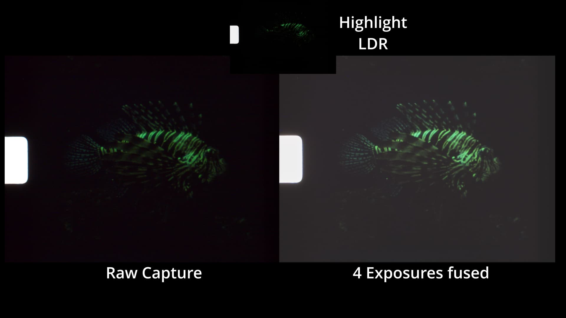
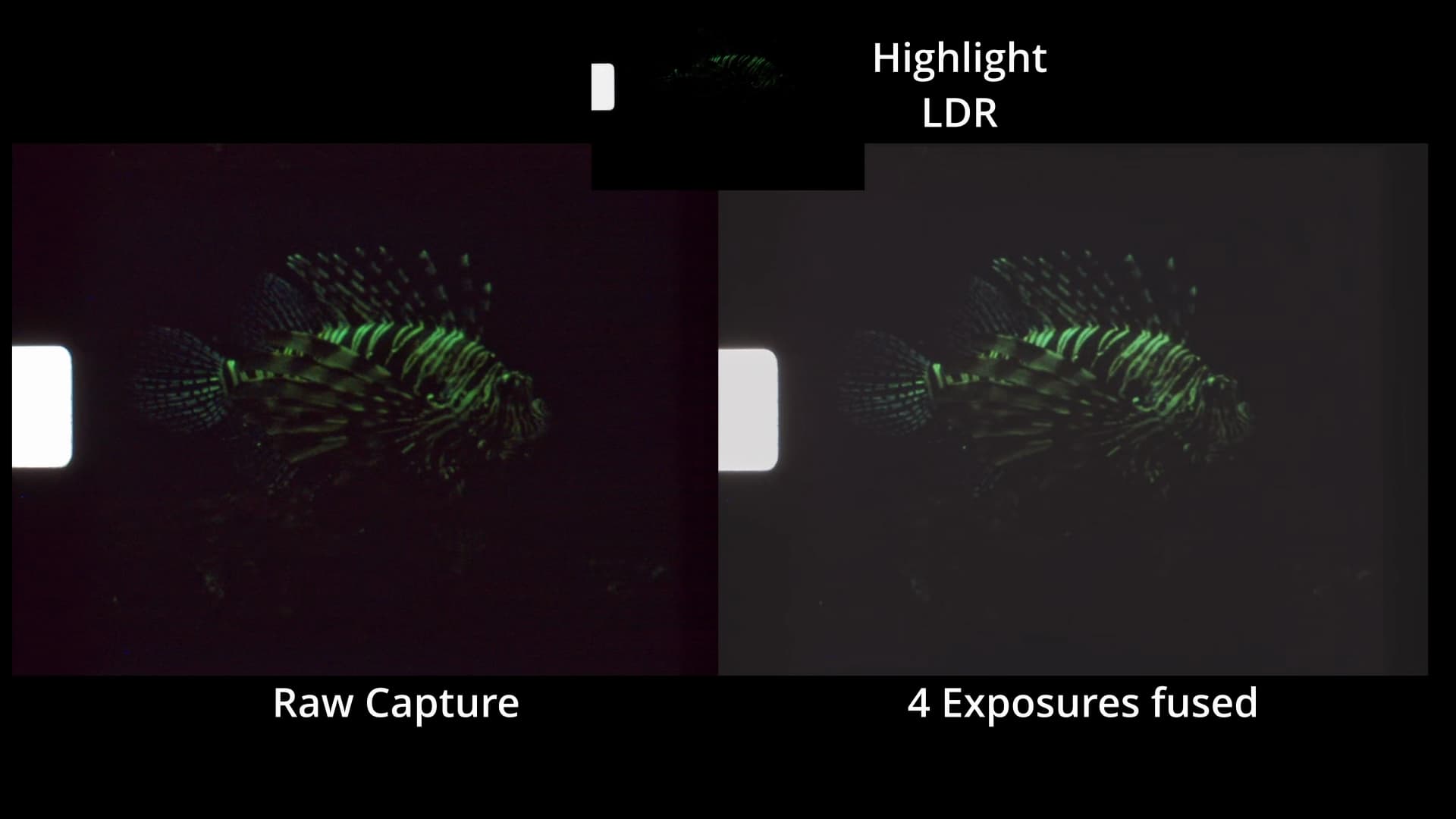
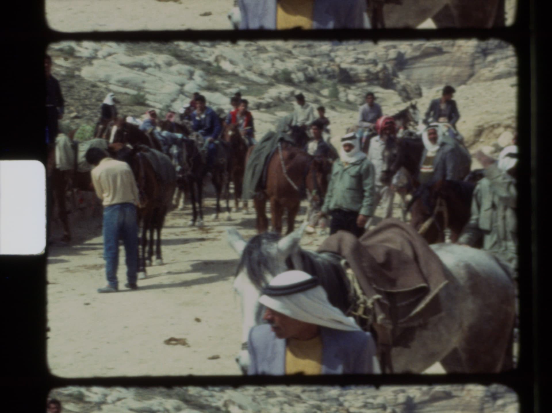
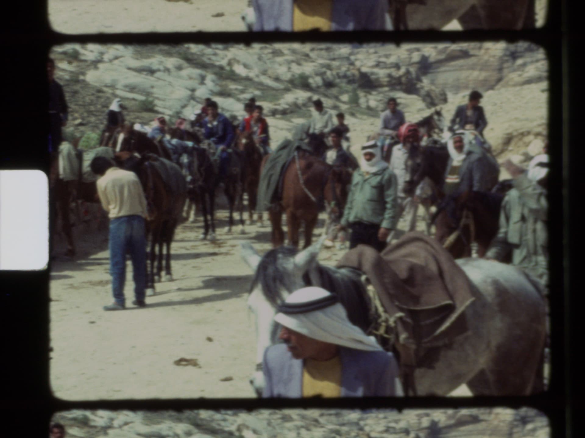
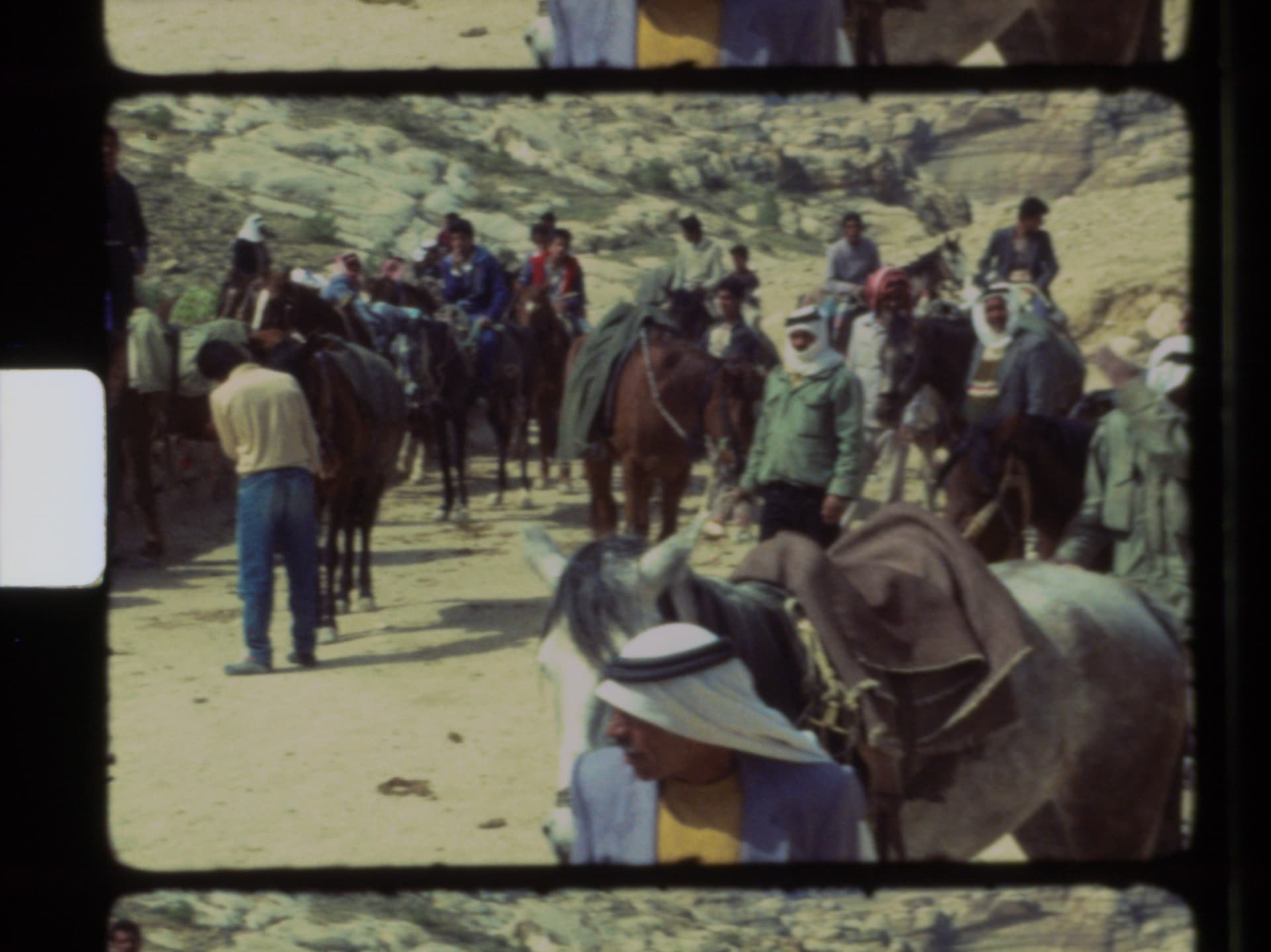
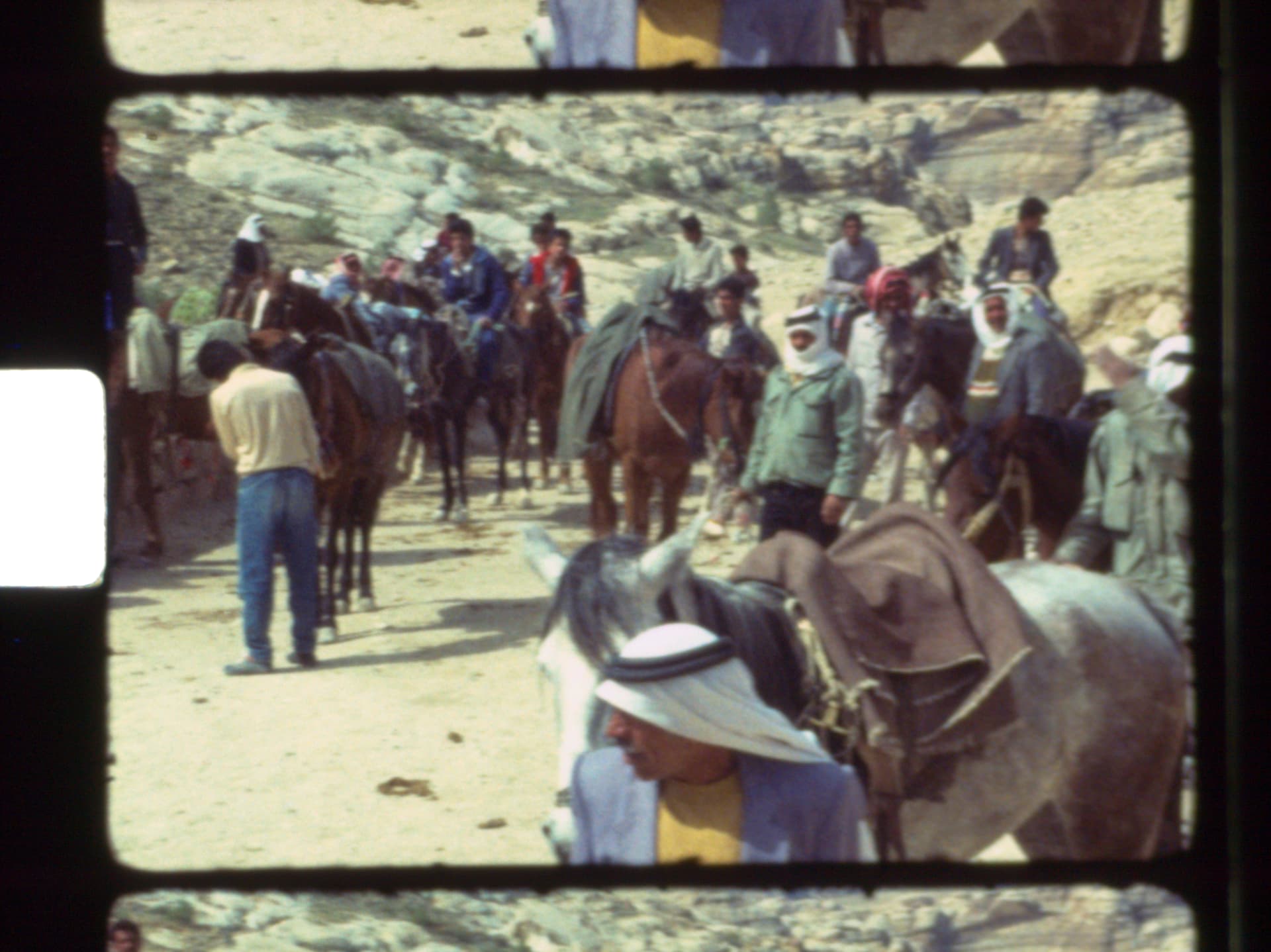
The 12-bit per channel dynamic range of the HQ sensor/camera is not sufficient to cover the range of densities one will encounter in small format color-reversal film. You will have problems in the very dark areas of your footage. Here’s some footage from the above scan to show [Edit: replaced the old clip with a clip using a higher bitrate] some more examples. (You absolutely need to download the clip and play it locally on your computer. Otherwise, you won’t see the things we are talking about. You should notice also some banding in the fish-sequences and a somewhat better performance of the raw in highlight areas.)

As remarked above, this scan was not optimal for raw capture. Improvements possible:

1. Work with an exposure setting so that burned-out areas of the film stock in question are at 98% or so of the total tonal range. One can get very close to 100%, as we are working in a linear color space (RAW). This is different from .jpgs which are non-linear by design and thus you have to be more conservative with the intensity mapping (I personally use the 93% mark, which is equivalent to a 240-level on an 8-bit per channel image).

2. Don’t push the shadows that much in those critical scenes. That’s an easy measure as you just have to accept that this limit exists in RAW capture mode. Done.

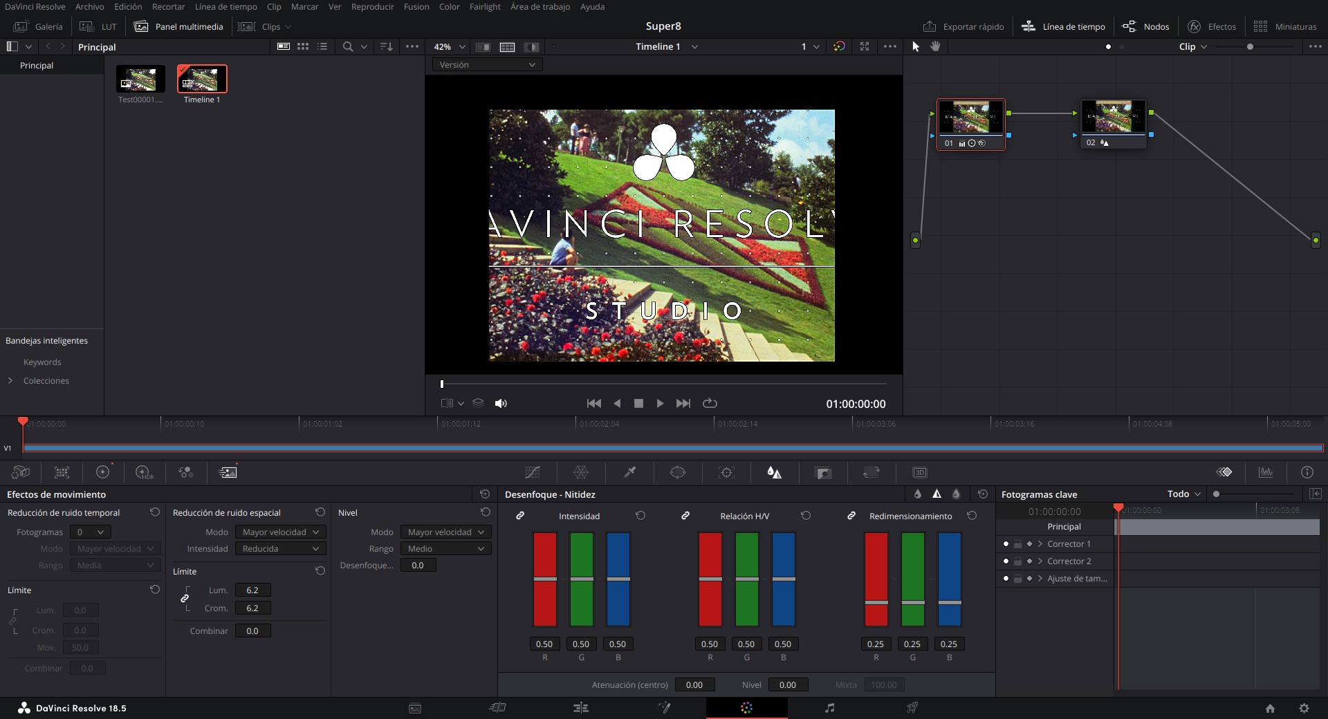
3. Employ noise reduction. There are two opposite positions out there: one states that “the grain is the picture”, the other one that “the content is the picture”. The later one potentially opens up the possibility of drastically enhancing the appearance of historic footage and should help with the low intensity noise of the RAW capture method as well. I will have to look into this with respect to RAW captures; here’s an example of what is possible on exposure fused material:

(To the right the original, noisy source, left and middle section slightly differently tuned denoising algorithms, A 1:1 cutout of an approximately 2k frame.)

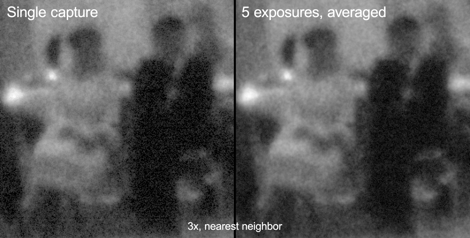
Another option to tackle the just-not-enough dynamic range of the HQ sensor is to combine several RAW captures into a higher dynamic range RAW. Two options have been discussed here:

1. @npiegdon’s suggestion of capturing multiple raws with the same exposure setting and averaging out the noise. The above example of @npiegdon shows that it works. The left image shows, if you look closely, the horizontal “noise” stripes, the right, averaged picture misses that “feature”.

2. @PM490’s suggestion of combining two or more raw captures with different exposure times to arrive at a substantially improved raw.

Both approaches might be quite feasible, as the HQ sensor delivers 10 raw captures per second, so there is plenty of data available for such procedures. Only writing the raw data finally as a .dng to disk slows down the whole procedure, taking about 1 sec per frame.

While you need quite a few captures for approach 1. (I think the 5 exposures @npiegdon used in his examples are somewhat a sweet spot), potentially, you only need 2 appropriately chosen exposures for approach 2. And the digital resolution achievable in the shadows would be better than in approach 1.

I’ve been running tests along these lines, albeit some time ago. Can’t really find any detailed information right now, have not kept enough records. Anyway, here’s the attempt to recover this:

First, the noise reduction in @npiegdon approach is related to the number of captures (assuming independent noise sources) to scale like one over the squareroot of the number of captures. So initially, you get an noticable advantage, but to improve things further, the number of captures increases. If you get a lot of images fast, that’s a great way to get rid of sensor noise. In the case of the HQ sensor, things are moving substantially lower - we get only 10 fps out of the sensor at 4k.

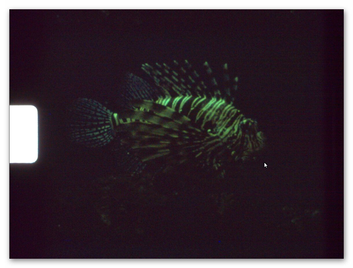
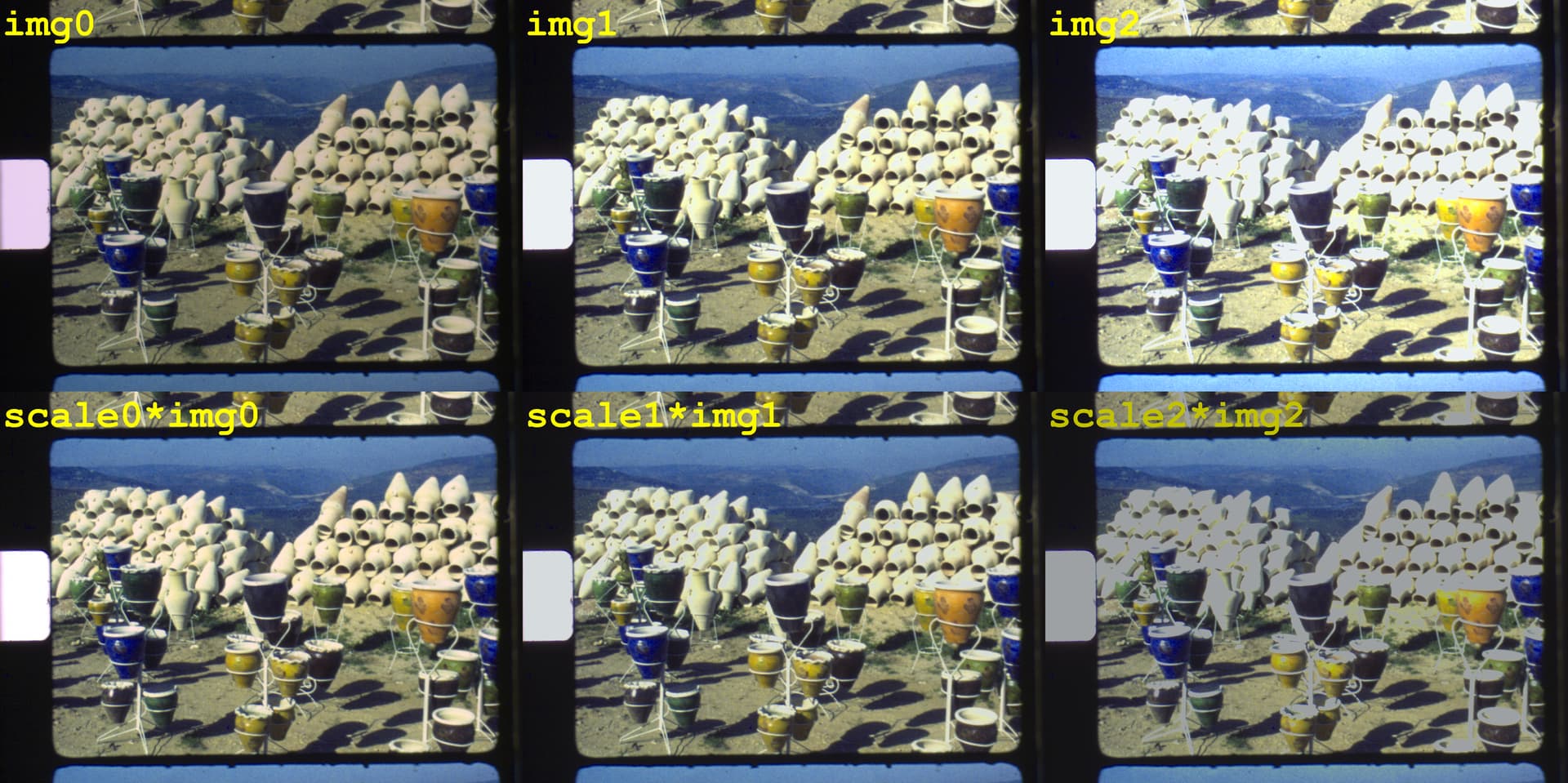
Secondly, with a few tricks the HQ sensor can be persuaded to rapidly switch exposure times. This opens up the possibility to capture a raw exposure stack and combine the captured raws somehow. The upper row of the following image shows three different raw captures (transformed with wrong color science to sRGB-images - that was done some time ago)

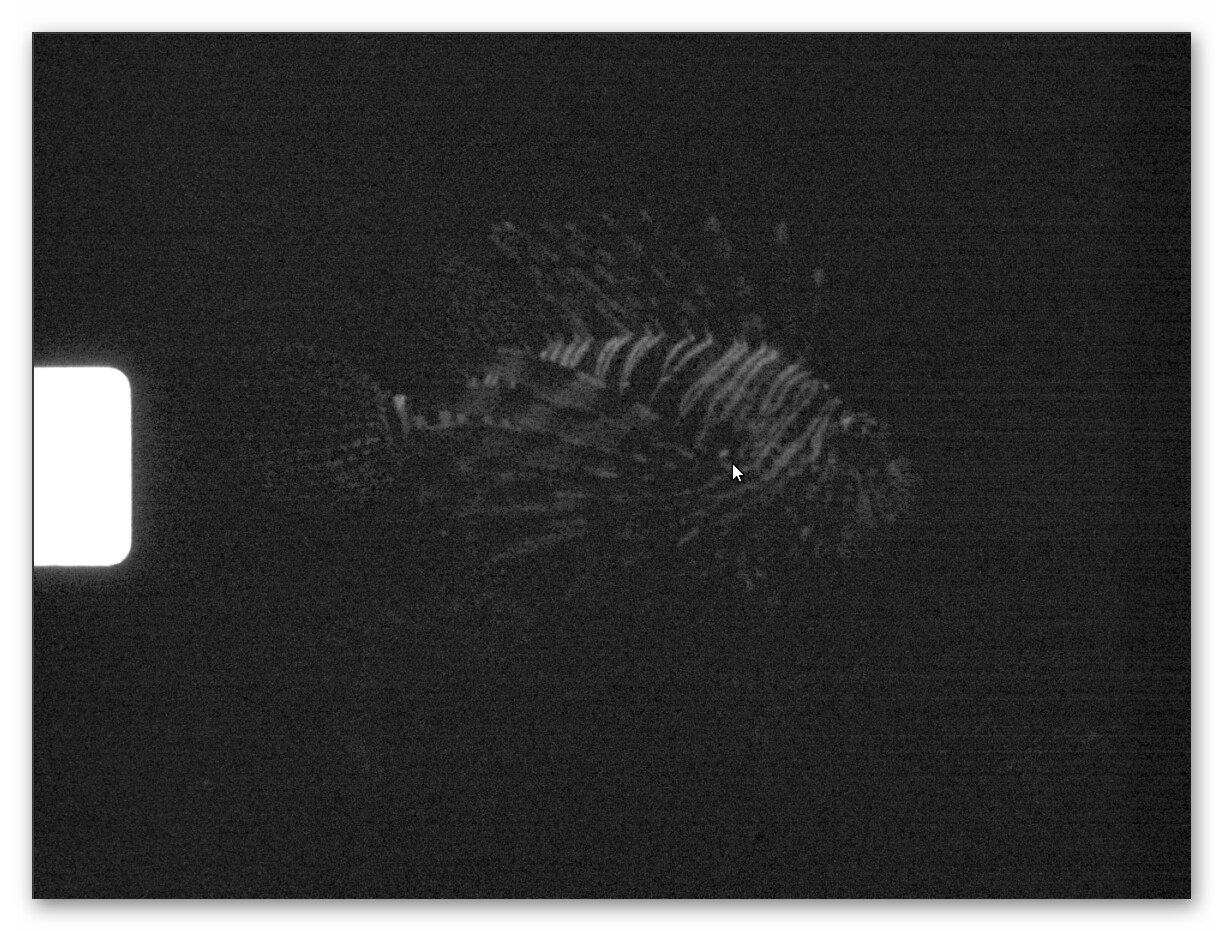
img0 is the classical “don’t let the highlights burn out” base exposure, the two other raw exposures are one f-stop brighter.

Since raw images are in a linear color space, alignment the data should be trivial, by appropriately chosen scalers. That’s what the lower row shows.

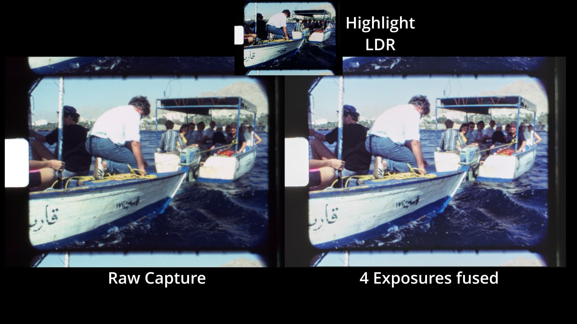
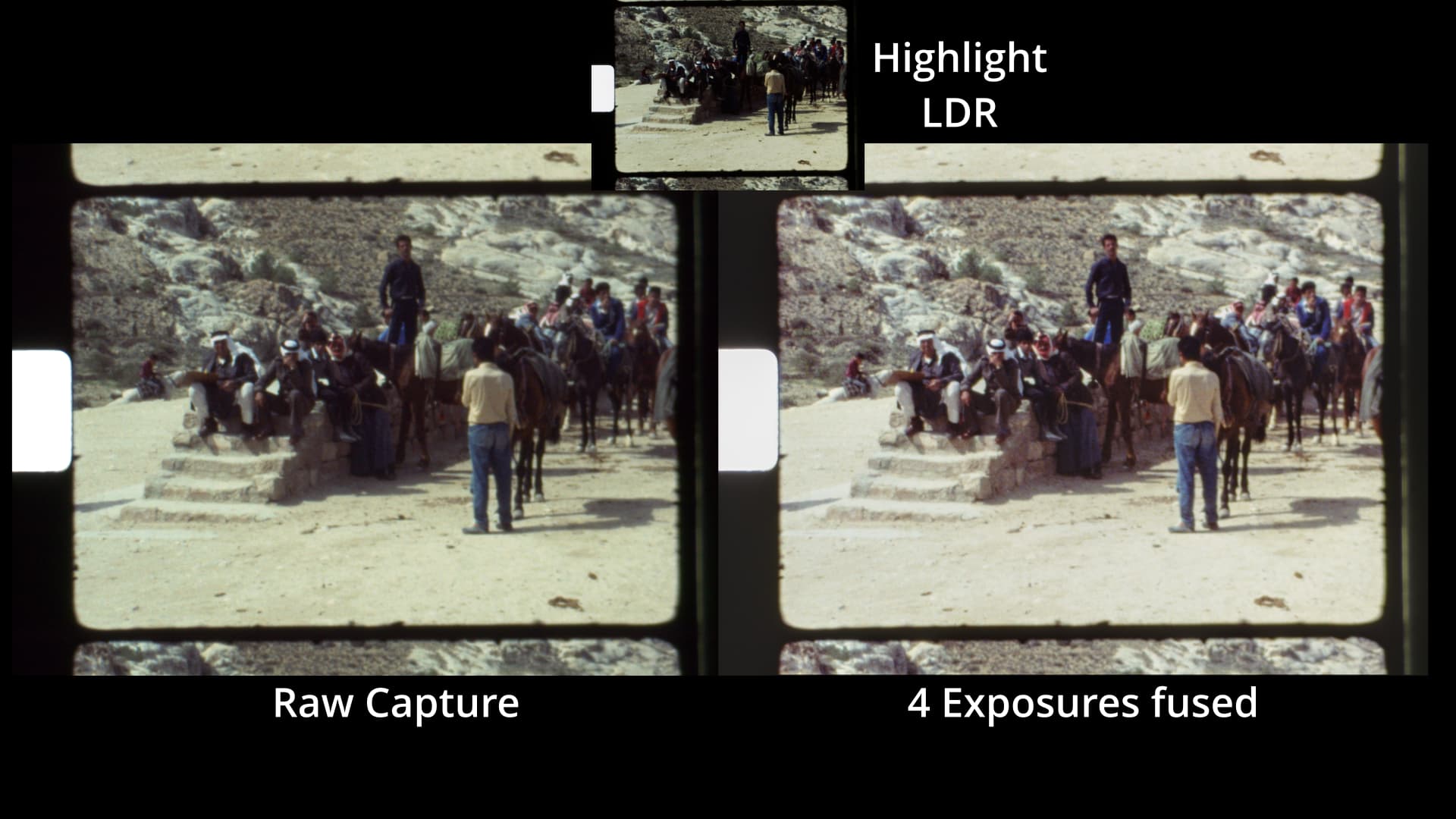
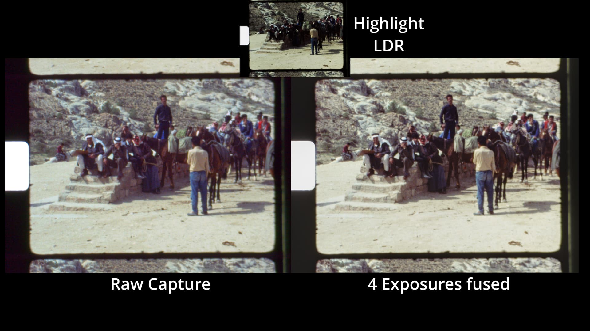
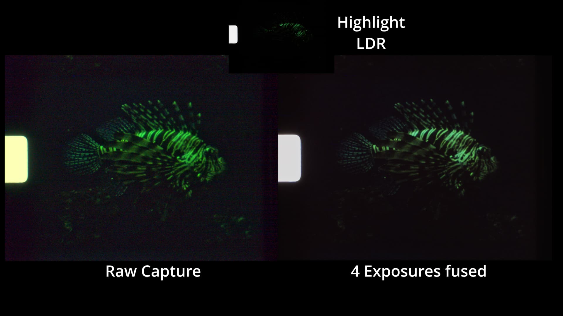
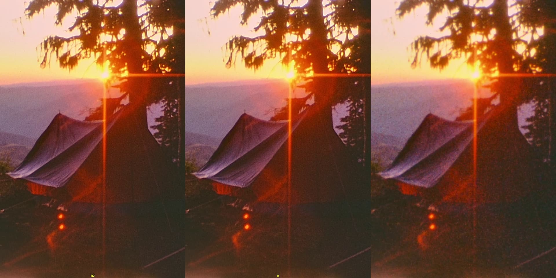
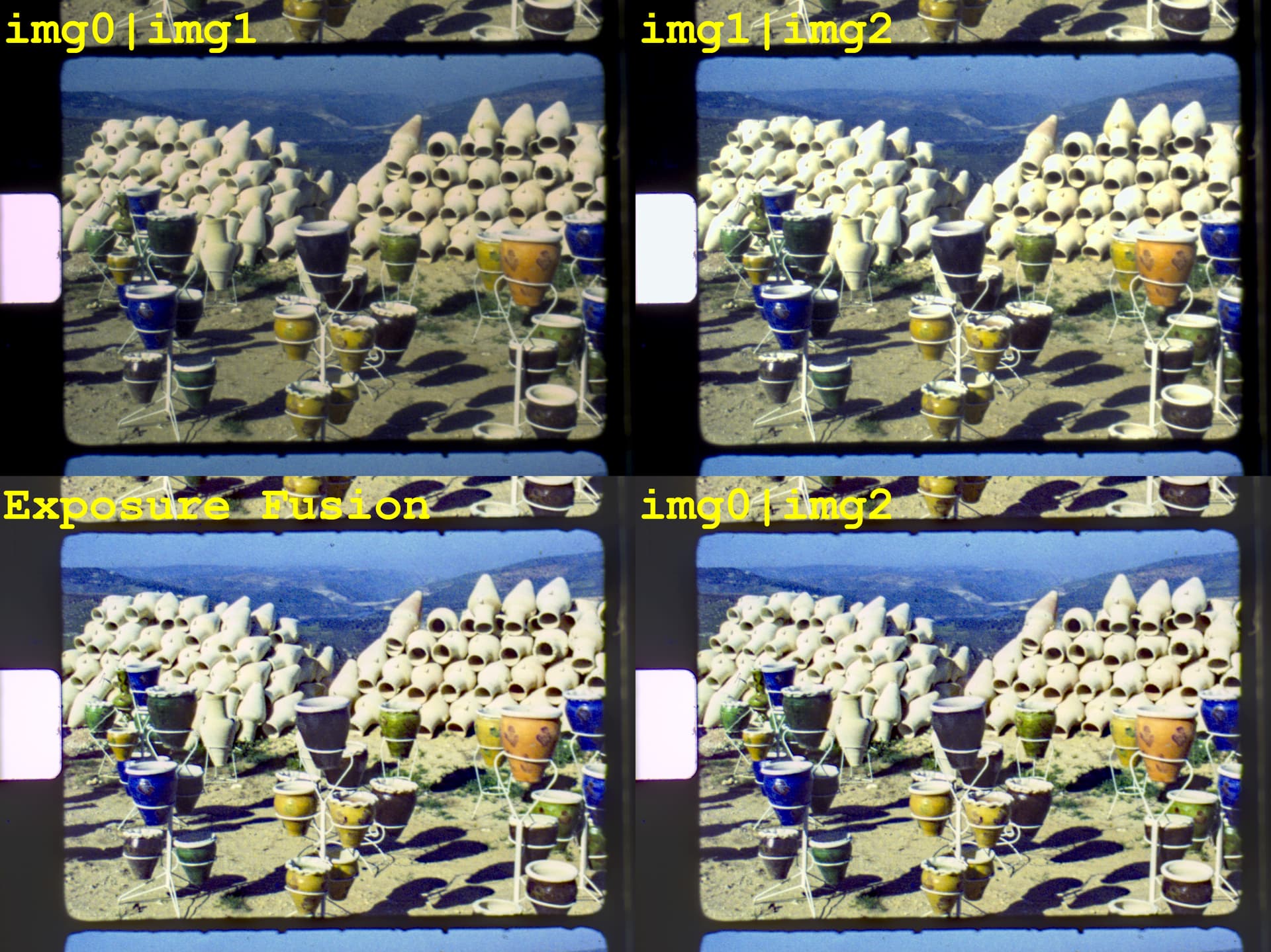
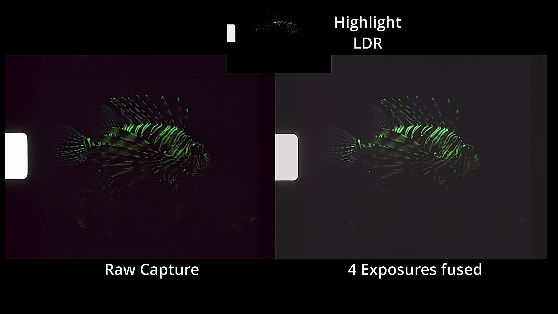
Here are the results I obtained at that time (note the exposure fused result in the lower left corner for comparision):

“img0|img1” indicates for example a combination of raw image 0 and raw image 1. You can not simply average both images together, as the blown-out areas of image 1 destroy the image structure in those areas. The images were combined differently: if the intensity of a pixel was above a certain threshold, data form the dark image was taken, if it was below that threshold, data was taken from the brighter image.

In this way, a good signal was obtained in shadow areas of the frame, with only two captures. However, in the vincinity of the threshold chosen, there was some slight banding noticable. Therefore, a second approach was tried - namely blending in a soft manner over a certain intensity range.

That blend needs to be optimized. You do not want shadow pixels from the dark raw image and you do not want highlight pixels from the bright raw image. I did get some promising results, but at the moment, I can’t find them. As at that time the color managment/raw handling of the picamera2 lib was broken, I did not continue that research further. One issue I have here with my scanner (because of the mechanical construction): there is a sligth movement between consecutive exposures, and I need to align different captures. Not that easy with raw data. This might not be an issue with your scanner setup.

Anyway, I think it’s time now to resurrect this idea. Getting two differently exposed raws out of the HQ sensor will take about 0.2 sec; storing that onto an SSD attached to the RP4 will eat up 1 sec per frame, but because of my plastic scanner, I need to wait anyway a second for things to settle down mechanically after a frame advance. Potentially, that could result in a capture time of 1.5 sec per frame. I currently need about 2.5 sec for a 4 exposure capture @ 4k, so in fact the raw capture could be faster.

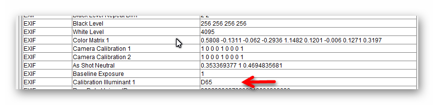
As far as I know, in the .dng-files picamera2 creates the color science is based on forward matrices Jack Hogan came up with. These are actually two matrices for two different color temperatures, one at the “blueish” part of the spectrum, one at the “redish” part.

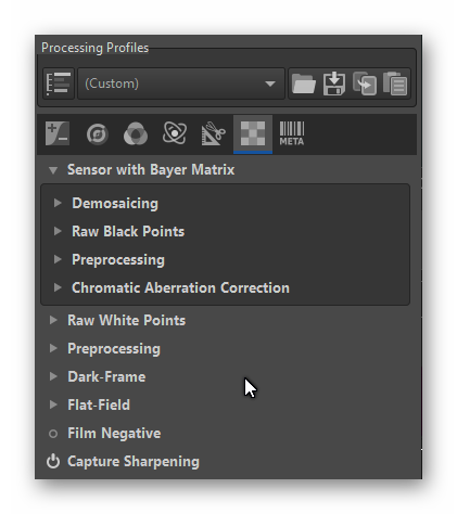
In your raw software, once you select “camera metadata” (or a similiar setting), the raw software looks at the color temperature the camera came up with and interpolates a new color matrix from the extreme ones stored in the .dng-file. Not sure whether the color temperature reported by the camera in the .dng-files is the correct one when using manual whitebalance (red and/or blue gains). I have to check this. That might throw off the colors.

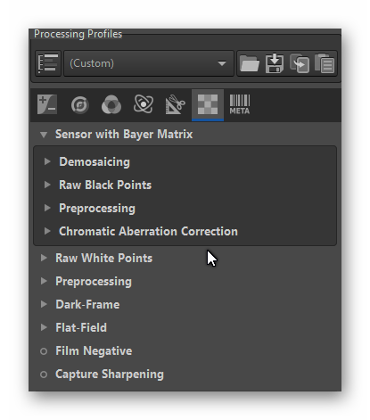
For people who are familiar with raw processing, there are additonal .dcp-files specifically for the HQ camera you might want to try when going from raw to developed imagery. You can find and download them from here.

If you use either the color matrices embedded in the camera’s metadata or the .dcp-profiles Jack came up with, you will always get an interpolated matrix, based on the current color temperature. Ideally, you would want to work with a fixed color matrix calibrated to your scanners illumination. That’s what I did until recently, when the Raspberry Pi foundation changed without annoucement the format of the tuning file. Currently, I am using the “imx477_scientific.json” tuning file for .jpg capture which features optimized color matrices for a lot more intermediate color temperatures. So, color science with the HQ camera seems still to be a mess - I did not yet have the time to sort this out.

So, wrapping up this long post: raw capture seems to have some advantages compared to exposure fusion, as well as some drawbacks. It seems that several raw captures combined in a super-raw might be the way to go forward. Raw captures record colors more consistently than the results of an exposure fusion; manually tuning highlight and shadows in raw captures seems to deliver the same or better results than the automatic way exposure fusion is doing. There are issues in the dark parts of raw captures - they limit what you can do in the post. Alternative approaches like combining several raw captures into a super-raw might be feasible, depending in part on the mechanical stability of your scanner.

[cpixip]

ok… - I realized that already the compression used to create the above linked video file eleminated some of the noise present in very dark areas of the RAW footage to a certain extent.

So, here’s another try, which should show the noise and the horizontal banding slightly better (I have replaced the link above also with the higher bitrate version).

Now, I ran this footage through one of my degraining scripts for a quick and dirty test. And indeed, I have trouble to notice any noise or banding in the result.

So, point 3. above, “employ noise reduction”, seems to me to be an integral component of the single RAW capturing approach. Given, one operates just at the verge of a cliff (sensor noise creeping into the image), but I think the approach is usable - with only a single RAW capture.

[Note: this is really a quick-and-dirty test - the degraining script normally expects pre-stabilized imagery (which I did not bother to use) and a certain minimum image size (>2k) (which I undercut with this footage). Nevertheless, I think in a real test with the full processing pipeline, the results will be similar.]

Here are two screen grabs out of the above linked videos. First the version with slight noise/banding:

and here the same frame, degrained

for direct comparision.

[cpixip]

– some more thoughts about using RAW captures taken with a HQ sensor.

The raws the picamera2 software is outputing are somewhat interesting. They claim to be DNG Version 1.4.0.0 - which is an old version of the DNG-spec. But, they are somewhat special.

Normally, dng-files carry with them two different sets of color information at two different color temperatures (warm, tungsten lamp like, and “daylight” D65). The color information consists of a ColorMatrix, a ForwardMatrix and the specification of the CalibrationIlluminant (“D65”, for example). As far as I understand it currently, a typical raw converter will take the “AsShotNeutral” tag - which is basically the color temperature and color tint your camera came up with, compute the color temperature at the time of exposure and interpolate the color matrices used in the transformation of the raw towards a real image from the two set of color matrices enclosed in dng-file.

Now, looking at the information contained in a HQ/picamera2 raw file,

one discovers that only one ColorMatrix1 is present (marked with the mouse cursor). The whitebalance data is there, as AsShootNeutral tag (these are the inverse gains which I set manually to fixed values in my scanner) as well as the CalibrationIlluminant1 (red arrow).

In a normal dng-file, you would find additionally ColorMatrix2, ForwardMatrix1, ForwardMatrix2 and CalibrationIlluminant2. So what happens here?

Well, first of all, such a simple dng-file is perfectly valid. Whether the specific raw converter you are going to use will interpret it correctly is another matter. More on that later on. I tried RawTherapee 5.8 as well as daVinci and did not get too weird results.

I asked David Plowman (the developer of picamera2) where the data in the dng-file is coming from. It seems to be that, as already remarked above, at least in the current version of picamera the AsShotNeutral-tag displays just the inverted red, green and blue gains (with green being always 1.0). The ColorMatrix1 is interesting: this is the matrix libcamera came up with during the capture. In auto whitebalancing mode, this would be a matrix interpolated from the tuning file data, based on the color temperature: the real matrix should be an interpolation between the most closely located color matrices in the tuning file (several matrices for different color temperatures are stored in this file). However, what libcamera/picamera does when color gains are set manually (the standard usecase in scanning applications) I still have to find out.

Why does it matter? Because any raw converter opening a HQ dng-file has only a single option: use the AsShootNeutral tag together with the given ColorMatrix1 to open the file. Since the origin of the numbers in the ColorMatrix1 data is yet unknow, the color science of an HQ dng-file is still somewhat arbitrary. Whether this really matters I will discuss a few lines below, stay with me.

I first want to remark that there is an alternative to using the color data embedded in the dng-files for developing the raws. That is: use a specially tuned input profile. I was not able to find out a way to convince daVinci to use input profiles, but any other raw converter can do it. So to use this approach with daVinci, you first need to batch-convert the raws into an intermediate format (linear tiff or png, for example) and load this into daVinci. That might be a faster approach anyway.

Well, continuing. Jack Hogan came up with these files for the HQ sensor and they can be downloaded from here.

I the following are examples created with RawTherapee 5.8. Dcp input profiles feature normally 0color information for two instead of one color temperature; the more advanced ones have also been manually tuned to give better results.

First, this here is the result using the color data embedded in the dng-file, that is, using “Camera standard” in the “Color Management” section of RawTherapee:

The simple “PyDNG_profile.dcp” features optimized color matrices for two color temperatures; to activate it, you have to activate the “Custom” selection in the “Color Managment” section of RawTherapee and load “PyDNG_profile.dcp”.

There are differences, but they are minor. So the simple dng-format picamera2 is producing is not too far off from Jack Hogan’s two matrices approach. Note the this specific capture was done with the “imx477_scientific.json”. The results will probably differ if you are using the standard tuning file for capturing.

Anyway, now on to a more elaborated dcp. I used the " Raspberry Pi High Quality Camera Lumariver 2860k-5960k Neutral Look.dcp" one. Here’s the result:

Now, that is a difference, color-wise. The reason is the additional “Look table” embedded in this profile. In fact, if you are adventurous and try this out with your own raw files: you can activate and deactivate the various contributions in RawTherapee by selecting or deselecting the appropriate entries in the “Color Managment” section.

Finally in this parade, let’s have a look at the result simply using the dng-embedded color data (that is anyway the usecase when opening the raws directly in daVinci) and manually tuning the colors. Here’s the result (a RawTherapee result, not daVinci):

Still would need a secondary color grade, but already close to the film footage.

Looking back at all this, it seems that just loading the captured raws into daVinci and color grading is a feasible way to go. Even so the color science behind that is still kind of murky.

There are some additional points to consider which point into the same direction. First of all, we are talking about old footage. Various degrading might/will have happened which changed the colors in a way that heavy color grading is necessary in postproduction to achieve something viewable. So “exact” color science is probably just wishful thinking. Second, there is an intrinsic problem hidden in the technical design choices taken when this material was introduced. The film stock was designed to work with tungsten lamp like illumination. A second color temperature (“daylight”) was available by the use of daylight-filter build into the cameras. That was all. There were no other, intermediate color temperatures available like in today’s digital world. So in many situations, already at the time the footage was taken, the colors were off. With the color grading tools available nowadays (and daVinci easily outperforms here classical raw converters), we have the option to fine-tune every single take of a film roll, or keep the color variation between scenes, to approximate the look of the original footage.

[dgalland]

@cpixip

Secondly, with a few tricks the HQ sensor can be persuaded to rapidly switch exposure times …

What is that magic trick! I’ve never been able to get below three images to ignore after an exposure change. ?

[cpixip]

@dgalland - there are two design choices made by the libcamera team which makes the task of rapidly switching exposure times difficult:

1. they stole the old digital gain control from the user. They use the digital gain control nowadays for better approximating the exposure time the user requested. The reason: any sensor can only realize a specific, limited set of exposure times by itself (in hardware). With libcamera, the user is not restricted in the exposure values he requests, but libcamera approximates the requested exposure time by a nearby exposure time the sensor can actually produce in hardware, plus a second rescaling of the image’s intensity value by an appropriately chosen digital gain factor. In my opinion a bad design choice, but it’s baked into libcamera.

2. It takes ages for a command issued in your program to travel down the libcamera path to the real hardware level which actually implements the command. And it takes again ages for the result with the new parameter(s) to appear as captured frame finally in your program. Some time ago, I measured that delay and got about 11-13 frames delay until a parameter setting issued showed up in the photograph. So an exposure change at time = 0 will show up only at frame number 12, for example. With the HQ sensor running in 4k mode, that is a delay of more than 1 sec…

So here are now the tricks to counteract these bad design choices:

1. To get rid of the digital gain annoyance, simple find suitable exposure times which libcamera can realize directly in hardware, without employing the digital gain trick. I am far away from my code, but I think the exposure times 2400, 4800, 9600, and 19200 fulfill for example that requirement. Some time ago, libcamera still needed a few frames to realize that the digital gain for a specific exposure would end up at 1.0. (the lib took two, three or even more frames to come slowly to that conclusion - with the result of introducing a tiny flicker on captures done too early) - I think those times have been gone.
   
   The following trick won’t work if you just use arbitrary exposure times.

2. The long delay between requesting a parameter and getting the appropriate result can be handled by introducing two different loops.
   
   One loop simply cycles all exposure times needed and requests them in turn. So for a three exposure setting, you would
   
   1. at time = 0 request 2400
   2. at time = 1 request 4800
   3. at time = 2 request 9600
   4. at time = 3 request again 2400, and so on…
   
   After a delay of 11 to 13 frames, the metadata of your frames should start to cycle in the same pattern.
   
   At the receiving end of the camera pipeline, after a frame advance, you would monitor the metadata of the frames for the exposure value. As that receiving end is not synchronized, any of (in this case) three exposure values might show up. Let’s say it has a metadata tag of 4800. Fine, store it as second exposure. The next frame will be 9600, store this as third exposure. The next frame will have exposure metadata of 2400 (as this completes the cycle you are requesting from the camera). Store this as first exposure. Your list of exposures is empty now - advance to the next frame and do the whole step again.
   
   Note: this next frame capture might start with 2400, 9600 or again with 4800. Since the two loops are not synchronized, you never know which of the three exposures comes next. But the following (in this example) two exposures will be the ones missing for your full exposure stack.
   
   To get this approach fully functional, you need to include something like the following third step:

3. libcamera reacts faster than it used to do when adapting digital gain to the appropriate value. Nevertheless it is a good idea to check both exposure value as well as digital gain (both of them should be returned with the metadata of the frame) for the correct values. Only accept a frame if both exposure value and digital gain are within appropriate limits. For example, with requesting an exposure value of 2400, you can expect to get precisely this value. The digital gain should be exactly 1.0. But sometimes, this might not happen. You might get frames back with digital gain = 1.01, for example. That is bad, but sadly unavoidable with libcamera. That means that this frame is slightly brighter than a previous frame captured with a digital gain of 1.0. You just have to accept this. In fact, this difference of 0.01 is not really noticable in the captures.
   
   Anyway, you have to decide on a tolerance threshold for both exposure time and digital gain to accept a frame delivered - or reject it. If so, the above described algorithm would just retry to capture the missing exposure on a second or maybe a third exposure round. If you are asking for too thight parameters, you will never get a valid frame out of the camera. Some tests are in order to get this working.

I hope the above description is not too confusing. But an approach like this can result in quite fast exposure stack capturing. For example, if you wait a second after each frame advance to allow your scanner to settle mechanically, it takes at 4k resolution less than 0.4 sec to capture an exposure stack with three exposures. My scanner is currently working with 4 exposures; with a one second mechanical wait before each frame is captured and with transmitting that frame to a main-PC, I get about 1.8 sec capture time per frame.

All in all, I will probably switch in the near future to a single raw-based capture instead of capturing an exposure stack. The raw-approach seems to be so much easier and while it might operate on the edge for some challenging footage, for most footage is seems to work fine.

[Ljuslykta]

@cpixip

All in all, I will probably switch in the near future to a single raw-based capture instead of capturing an exposure stack. The raw-approach seems to be so much easier and while it might operate on the edge for some challenging footage, for most footage is seems to work fine.

I think it was touched upon earlier in the thread, but if a single raw capture isn’t able to capture the full dynamic range, wouldn’t the logic step to take one capture over ideal exposure setting for just one picture, then take one under. Next step, develop the RAWs to jpeg or png and do some sort of fusion on them. Or do we end up with the colour shift that was noticed when doing Mertens?

[cpixip]

@Ljuslykta

I think it was touched upon earlier in the thread, but if a single raw capture isn’t able to capture the full dynamic range, wouldn’t the logic step to take one capture over ideal exposure setting for just one picture, then take one under. Next step, develop the RAWs to jpeg or png and do some sort of fusion on them. Or do we end up with the colour shift that was noticed when doing Mertens?

Well, maybe its time to summarize the various options which are available with the HQ sensor, a sensor which delivers maximal 12bit per color channel.

Before that, let me just define a few things.

• exposure stack. a stack of captures taken with different exposures. Is normally done by changing the exposure time between captures but can also be achieved with varying the illumination between exposures.

• LDR image. LDR stands for low dynamic range images, that is, the image format features at most 8 bit per color channel. That implies a non-linear relationship between intensities the camera has seen (=raw, more than 8-bit) and the intensities coded in the image data (just 8-bit)

• LDR stack. . An LDR stack is a collection of differently exposed LDR images. A typical example would be a collection of four or five different exposures of a single frame, transmitted and stored as .jpg-file. The intensities coded in a .jpg-file are not linearly related to the image intensities (non-linear).

• RAW stack. The raw stack is also a collection of different exposures, but its intensities are linear coded and feature at least a bit depth of 10 bit, typically 12 bit (at this time up to 14 bits for expensive cameras). A collection of different raw captures of a frame with different exposure times would be a typical raw stack.

• HDR image. Literally, a high dynamic range image. An often misused term; in my opinion this term should be reserved and used only for image data which is linear in light intensities and can code every value imaginable. That is, each pixel can code an arbitrary and unrestricted floating point number. OpenEXR is such an format. To make the point: anything stored as a .jpg is not. Neither any other image format with 8 bits per color channel.

Picking up the last topic - how do we generate a real HDR? Well, one way is to capture a sufficiently large LDR stack, get rid of the non-linear relationship between pixel values and combine the now linearized LDR images in a way that the full dynamic range covered by the different LDR exposures is recovered. That is exactly what Paul Debevec’s algorithm does.

The HDR computed by Debevec’s algorithm is rather disappointing on displays we usually have available. The reason is the linear relationship between intensities and pixel values in the HDR image, as well as the fact that most of us probably only own a display operating with 8 bits per channel (i.e. a LDR-display). So to arrive at something you can show to your audience, you have to add a non-linear step which squashes the large range of values found in the typical HDR image into the small 8-bit range a standard display can work with. That step is called tone-mapping, and all automatic algorithms I am aware of fail in some way or the other.

Here comes the Merten’s exposure fusion algorithm to the rescue. This algorithm does not really care about HDR and so - it simply looks at the LDR stack and picks the data for each pixel from the LDR image which “looks best”. So exposure fusion maps a LDR-stack (non-linear) into a single LDR (non-linear as well) - without ever calculating a HDR image.

I think we are now in a position to discuss the various possibilities the HQ sensor combined with libcamera/picamera2 offers:

• single raw capture. Provided one captures in one of the 12 bit per channel modes, the dynamic range of the capture is sufficient to handle most scenes in Super-8 footage. Important is a proper exposure - the brightest image areas should be just a fraction below the maximal intensity (4095 or 98-99% in RawTherapee). A conservative measure is to use the sprockethole or the empty film gate for adjustment. A better option would be to use a clear area of the film stock you are about to scan to set the exposure time. Typically, a clear film reduces the light by about 10%.
  
  As shown already in this thread, this single raw can be directly loaded into daVinci or can be converted via Lightroom or RawTherapee into something which can be loaded into an edit program. With a little tweaking of the shadows and highlights, quite good and consistent results can be obtained. Problematic are very dark areas; here especially the red channel of the HQ sensor tends to display noticeable noise - this will be reduced if a spatio-temporal degraining algorithm is part of the processing pipeline.
  
  From an archival point of view, at most 12 bit of the film dynamic can be captured by a single raw. The following option is in this regard better:

• multiple .jpg-images (LDR-stack). Here, multiple different exposures are taken of a single frame and collected into a LDR-stack. Typically, these images use jpg-encoding (which is non-linear). With suitably chosen exposure times, the dynamic range of the capture is larger than the 12 bit a single raw can achieve.
  
  A displayable image can be computed from this exposure stack either through the combination of the
  Debevec algorithm (which computes a real HDR), followed by an appropriate tone-mapping step to arrive at a displayable LDR. Or, via exposure fusion, by going directly to a displayable LDR.
  
  The Debevec algorithm is more complicated, but it creates an intermediate HDR - which is actually the ideal archival copy of the film frame in question (with a potentially unlimited dynamic range). The exposure fusion is much simpler and generates superior imagery of single frames, compared to most tone-mapped imagery. The only drawback is that it does not ensure that the color science stays constant over time. In fact, I have the suspicion that it does not do this.

• multiple raw images. That could be an approach where you get the best of both worlds. I did quite some time ago some experiments in that direction, but did not follow them through due to the weird colors I got at that time from raw imagery. These things have improved now.
  
  As raw sensor images are linear by definition, these things are in fact easy to combine. There should be no color shifts if done correctly. The combination basically results in a “super-raw” which can easily achieve 16 bit or more per color channel. Several options are here available:

  • define thresholds. Below a certain threshold, the lesser noisy data from a raw capture with higher exposure time is used. I tried this as a simple approach, but there was slight banding noticeable at the threshold values chosen.
  • smoothly interpolate band of values. Smoothly interpolate between the values of several raw captures. I tried this as well, and the results were visually better. How you interpolate the raw values and in which bands you do this is something I did not put much work into - here a lot of room for experiments is still available.
  • use Debevec’s algorithm. This algorithm is generic enough so that it should work also on raw data. One part of this algorithm estimates gain curves - these should in fact turn out to be a simple linear function in the case of raw data and could be used as a safety check that the calculations were done correctly. I have not tested this yet, but it seems to be an interesting option. You would end up not only with a “super-raw”, but also with a great archival real HDR.

Note that one specific algorithm can’t be used for the combination of raw images. It’s the exposure fusion algorithm - the intrinsic reason is that the exposure fusion algorithm is combining “good-looking” parts of the various exposures. But in a raw image, you do not have any “good-looking” parts (try to view it without being processed by a raw converter). Besides, you still would have the color-shifting effects which seem to be an intrinsic property of the exposure fusion algorithm. So exposure fusion of raw images is probably not a good idea.

Some final thoughts about this. Doing multiple exposures and combining them in some way requires that your scanner holds the frame absolutely stable during the exposures. At least with my scanner, this is not the case. So there is an additional, absolutely necessary alignment step in my processing pipeline. Switching from multiple exposures to a single one helps here tremendously, speeding up the capture process as well. That’s one of the advantages I see in the “capture a single raw” approach discussed here.

If you are anyway capturing a raw stack, it is probably of advantage to combine the raws already during the capture into a single new raw, before writing this raw image to disk. Storing a raw image takes about a second on the Raspberry PIs. Such an approach would favor simple combination schemes like the threshold or banding approach described above, but would probably rule out the direct application of Debevec’s algorithm - that would take too long to compute. However, a simplified version might be fast enough. Lot’s of things to try out, but I think I personally will stick to a single raw capture for now.