Ok, here’s the attempt of a short summary. In traditional analog photography, your reference point of exposure of normal (negative) film were the shadows. In contrast to this, with color-reversal film, you would set your exposure to image the brightest areas of your scene correctly, ignoring the shadows.
Now, with a digital sensor, you work like in the old days with color-reversal film. The simple reason - anything overexposed is lost forever. In the shadows, you can raise intensity levels digitally a little bit without too much compromises with respect to noise.
If you are doing automatic exposure with your DSLR (as a profi, you don’t), it is a good idea to underexpose the full frame a little bit - this makes sure that you have some headroom in the very bright image areas. But again, the professional way of exposure in the case of digital sensors is to choose an exposure time which brings the brightest image areas very close to the upper limit of the sensor (the whitelevel tag in your .dng). Because the bright areas are just below that limit, they certainly contain structure, that is, they are not burned-out. This maximal exposure also raises a little bit the shadow areas above the noise floor. So all good there too.
Any raw development program can only work with what the sensor did record, so you want to optimize the situation right at the sensor as best as possible. That is: you want the largest dynamic range you can possibly obtain. Since in the case of a film scanner the setup is fixed, as compared to usual DSLR photography, you can tune your exposure very precisely. That’s what you should do. The occasional advise with DSLRs to underexpose is just a little safety net to make sure the highlights do not burn out on an exposure based on image averages. This is not what you need or should employ in the case of film scanners.
The horizontal noise stripes mostly in the red channel have been discussed before. When spatio-temporal averaging is employed, these artifacts are also substantially reduced. Averaging 8 or more exposures is one option, another would be to employ denoising techniques similar to the ones discussed in the " Comparison Scan 2020 vs Scan 2024"-thread. But: try first to get your exposure in the right ballpark. In this respect:
Well, standard software like RawTherapee can give you some hints. If you just load the raw image into the program and leave the exposure slider on its default value, you should be able to use the histograph graph for an analysis. Let’s assume this capture
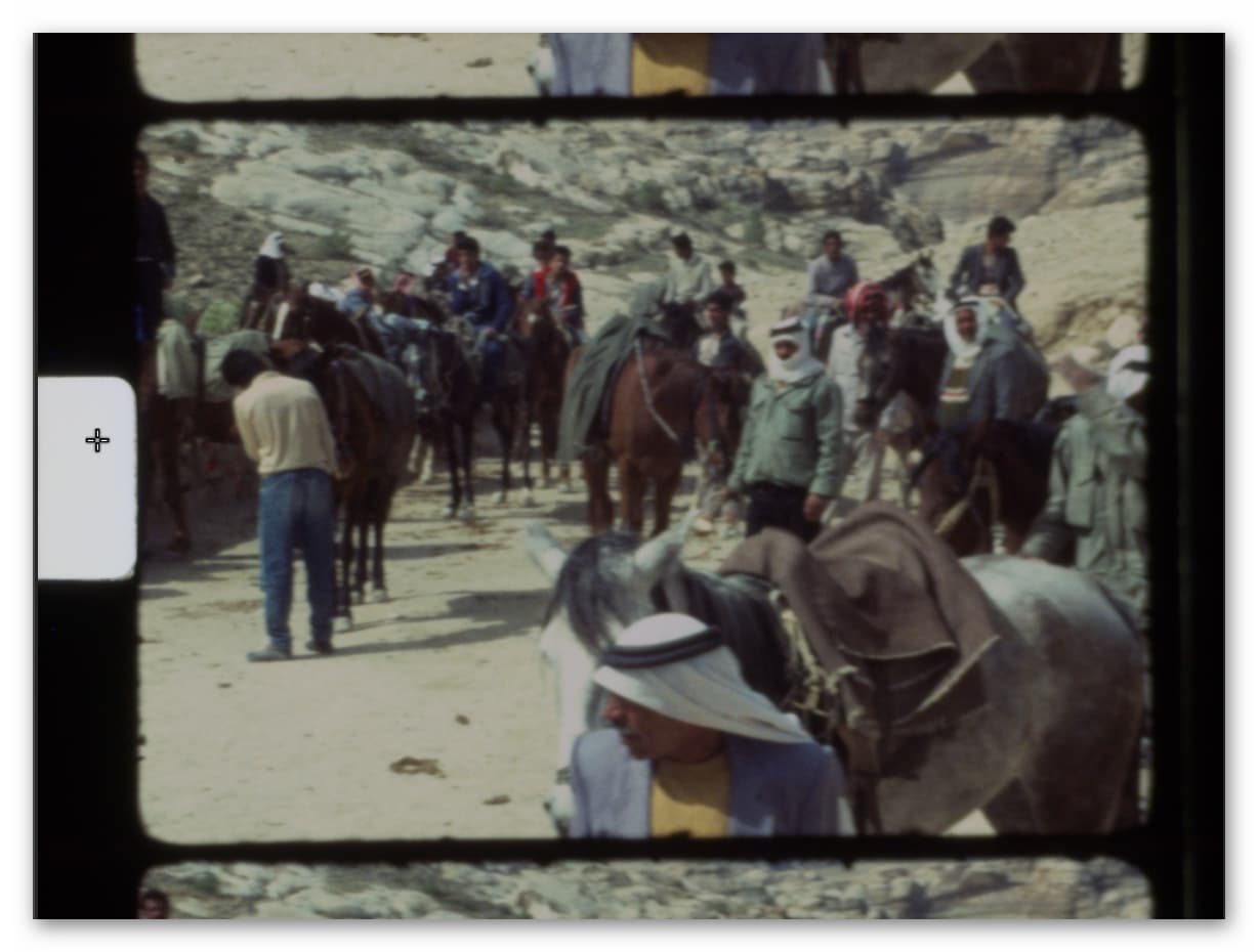
which is underexposed. The cursor is placed into the sprocket area. In this case, the histogram
shows us the following:
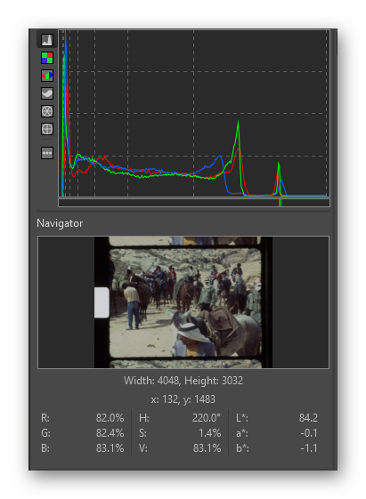
The tiny colored lines in the bar shows us the values of the current pixel - which is clearly only placed at a fraction of the range available. Indeed, as the value panel below indicates, the brightest area in the image is only a little bit above 80% of the full range. Bad exposure…
Here’s a simple Python program you could use as well:
import numpy as np

import rawpy

path = r'G:\xp24_full.dng'

inputFile = input("Set raw file to analyse ['%s'] > "%path)
inputFile = inputFile or path

# opening the raw image file
rawfile = rawpy.imread(inputFile)

# get the raw bayer
bayer_raw = rawfile.raw_image_visible

# quick-and-dirty debayer
if rawfile.raw_pattern[0][0]==2:

    # this is for the HQ camera
    red    =  bayer_raw[1::2, 1::2].astype(np.float32)                                 # Red
    green1 =  bayer_raw[0::2, 1::2].astype(np.float32)                                 # Gr/Green1
    green2 =  bayer_raw[1::2, 0::2].astype(np.float32)                                 # Gb/Green2
    blue   =  bayer_raw[0::2, 0::2].astype(np.float32)                                 # Blue

elif rawfile.raw_pattern[0][0]==0:

    # ... and this one for the Canon 70D, IXUS 110 IS, Canon EOS 1100D, Nikon D850
    red    =  bayer_raw[0::2, 0::2].astype(np.float32)                                 # Red
    green1 =  bayer_raw[0::2, 1::2].astype(np.float32)                                 # Gr/Green1
    green2 =  bayer_raw[1::2, 0::2].astype(np.float32)                                 # Gb/Green2
    blue   =  bayer_raw[1::2, 1::2].astype(np.float32)                                 # Blue

elif rawfile.raw_pattern[0][0]==1:

    # ... and this one for the Sony
    red    =  bayer_raw[0::2, 1::2].astype(np.float32)                                 # red
    green1 =  bayer_raw[0::2, 0::2].astype(np.float32)                                 # Gr/Green1
    green2 =  bayer_raw[1::2, 1::2].astype(np.float32)                                 # Gb/Green2
    blue   =  bayer_raw[1::2, 0::2].astype(np.float32)                                 # blue

else:
    print('Unknown filter array encountered!!')

# creating the raw RGB
camera_raw_RGB = np.dstack( [red,(green1+green2)/2,blue] )

# getting the black- and whitelevels
blacklevel   = np.average(rawfile.black_level_per_channel)
whitelevel   = float(rawfile.white_level)

# info
print()
print('Image: ',inputFile)
print()

print('Camera Levels')
print('_______________')
print('             Black Level   : ',blacklevel)
print('             White Level   : ',whitelevel)

print()
print('Full Frame Data')
print('_______________')
print('             Minimum red   : ',camera_raw_RGB[:,:,0].min())
print('             Maximum red   : ',camera_raw_RGB[:,:,0].max())
print()
print('             Minimum green : ',camera_raw_RGB[:,:,1].min())
print('             Maximum green : ',camera_raw_RGB[:,:,1].max())
print()
print('             Minimum blue  : ',camera_raw_RGB[:,:,2].min())
print('             Maximum blue  : ',camera_raw_RGB[:,:,2].max())

dy,dx,dz = camera_raw_RGB.shape

dx //=3
dy //=3

print()
print('Center Data')
print('_______________')
print('             Minimum red   : ',camera_raw_RGB[dy:2*dy,dx:2*dx,0].min())
print('             Maximum red   : ',camera_raw_RGB[dy:2*dy,dx:2*dx,0].max())
print()
print('             Minimum green : ',camera_raw_RGB[dy:2*dy,dx:2*dx,1].min())
print('             Maximum green : ',camera_raw_RGB[dy:2*dy,dx:2*dx,1].max())
print()
print('             Minimum blue  : ',camera_raw_RGB[dy:2*dy,dx:2*dx,2].min())
print('             Maximum blue  : ',camera_raw_RGB[dy:2*dy,dx:2*dx,2].max())
If you run it, the following output would be created by it:
Set raw file to analyse ['G:\xp24_full.dng'] > g:\Scan_00002934.dng

Image:  g:\Scan_00002934.dng

Camera Levels
_______________
             Black Level   :  256.0
             White Level   :  4095.0

Full Frame Data
_______________
             Minimum red   :  249.0
             Maximum red   :  1202.0

             Minimum green :  248.5
             Maximum green :  2839.0

             Minimum blue  :  245.0
             Maximum blue  :  1533.0

Center Data
_______________
             Minimum red   :  254.0
             Maximum red   :  892.0

             Minimum green :  264.0
             Maximum green :  1946.0

             Minimum blue  :  256.0
             Maximum blue  :  1096.0
First, it lists the black and white levels encoded the raw file. Ideally, these correspond to true black and maximum white - in reality, they not always are correct. This image was captured with a RP4, so the values are the original ones of the HQ sensor. A black level of 254 and white level of 4095 (=2**12-1).
The next section lists the minimal and maximal values found by analysing the full frame. Not surprisingly, the maximal value encountered is 2839 (in the green channel), much less than the maximal possible value 4095. (The minimal values found are slightly less than the black level reported by the sensor, but that is quite usual.)
The next section spits out the same information, but only for the central region of the image (without the sprocket region). Here, the maximum value found is even lower, at 1946 units. So again, this example raw is severly underexposed.
Here’s another example:
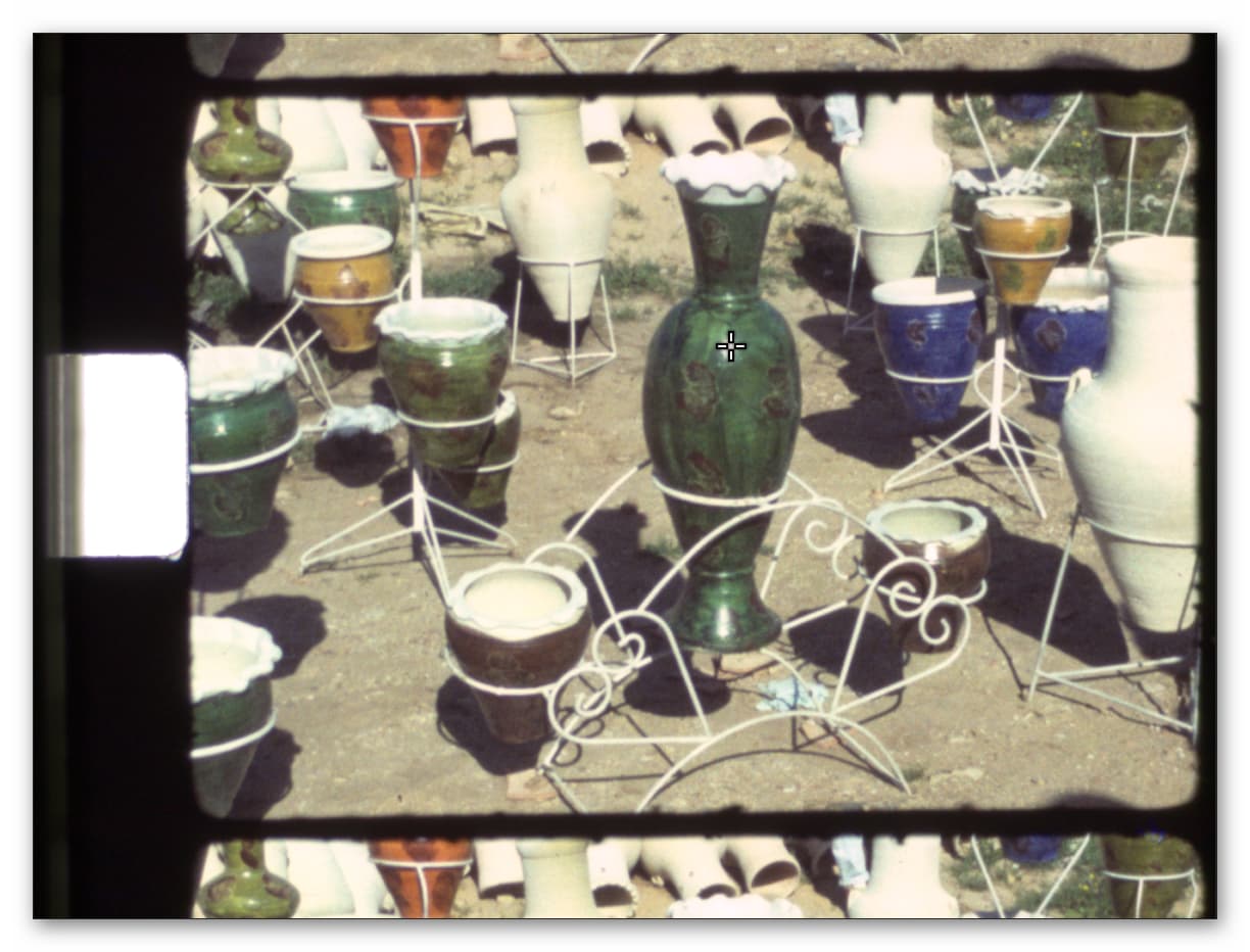
The testcursor is placed directly onto a highlight within the frame. The exposure value here is certainly less than the exposure value recorded in the sprocket hole. Simply because even the clearest film base eats away some light. Looking again at the histogram display:
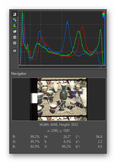
we indeed get for our test point RGB-values very close to 100%, but slightly below. This is an example of a perfectly exposed film capture.
Running the above listed python script yields the following output:
Set raw file to analyse ['G:\xp24_full.dng'] > g:\RAW_00403.dng

Image:  g:\RAW_00403.dng

Camera Levels
_______________
             Black Level   :  4096.0
             White Level   :  65535.0

Full Frame Data
_______________
             Minimum red   :  4000.0
             Maximum red   :  36896.0

             Minimum green :  4088.0
             Maximum green :  65520.0

             Minimum blue  :  3936.0
             Maximum blue  :  49152.0

Center Data
_______________
             Minimum red   :  4384.0
             Maximum red   :  26208.0

             Minimum green :  4936.0
             Maximum green :  63136.0

             Minimum blue  :  4384.0
             Maximum blue  :  32384.0
We see that the black level now sits at 4096 units and the white level at 65535. The image was captured with the HQ sensor as well, but processed and created by a RP5 - and the RP5 rescales the levels to the full 16-bit range.
Anyway. The “Full Frame Data” (which includes the sprocket hole) indicates that indeed we end up very close to the maximum value (65520 vs. 65535 in the green channel). Even in the central image area we reach 63136, which is very close to the maximal possible value, 65535. This is an example of a correctly exposed film scanner image.
Hope this clarifies a little bit what I am talking about. Again - the discussion concerns only the intensity values the HQ sensor is sensing. And it is our goal to optimize that range as good as possible. These values have nothing to do with any funny exposure adjustments your raw converter might throw upon the raw data. That is a secondary story.