I think it’s about time to close this thread. A lot of interesting discussions were triggered and I want to summarize what I can remember of these discussions, distributed among various threads and over quite some time.
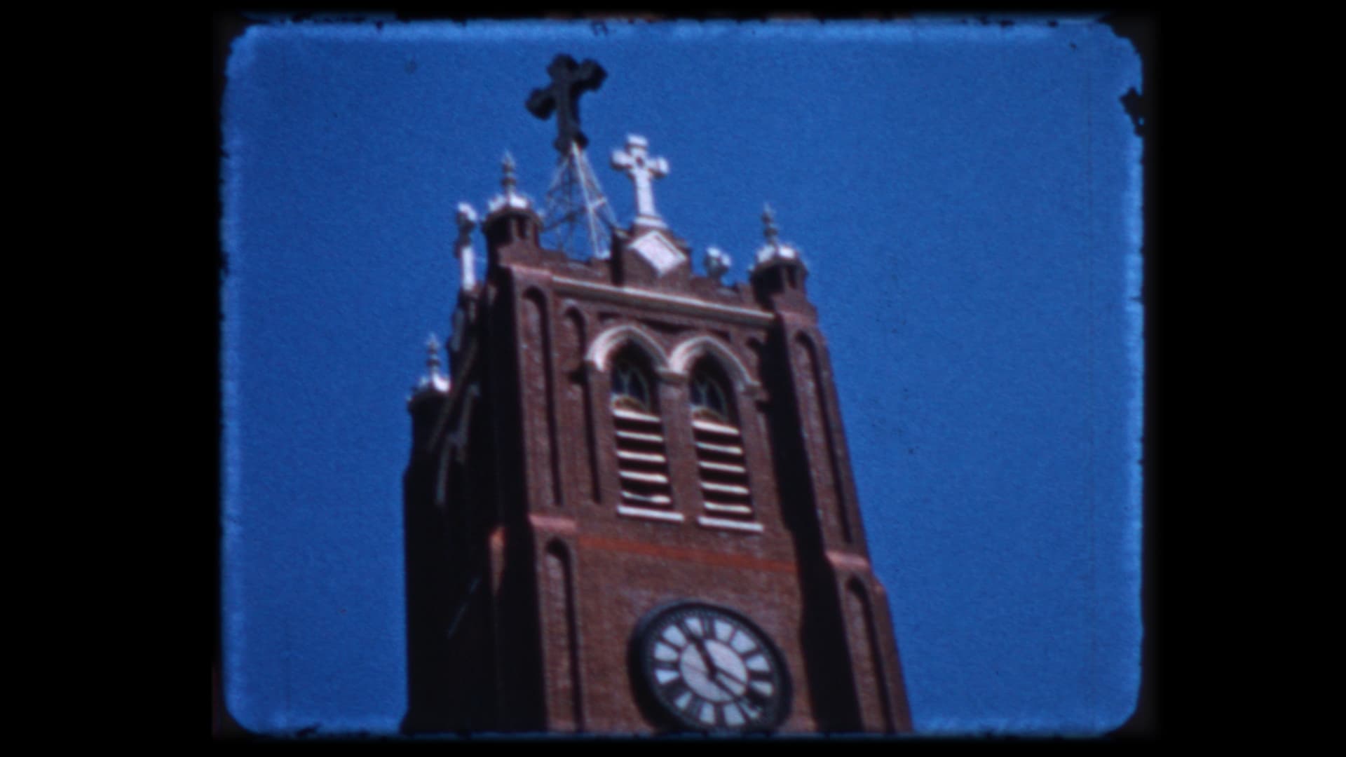
To recap: initially, the question was where the dark band in the red channel of a peculiar frame capture was coming from (the dark band in the sky):
It turned into a discussion about the origin of annoying noisestripes in captures done with the HQ sensor (which was also used in the capture example above), among other things.
While both issues are related, the causes are different. I will discuss that in detail in what follows. In short, the dark red band is caused by out-of-gamut colors - the HQ sensor is able to “see” colors which can not be represented in rec709 (or sRBG) color gamuts. The noisestripes however are an intrinsic property of the IMX477, the “camcorder” chip used in the HQ camera. But they are amplified by the color transformations necessary to arrive at correct colors.
Work-arounds in case of the out-of-gamut issue include:
- reduce saturation during capture, increase again in postproduction.
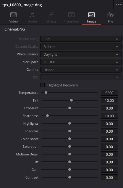
- just pretend that your raw format works in a larger color space (helps with DaVinci, for example). Easy, but colors are slightly wrong.
- maybe in the future: creating a tuning file natively working in a larger color space than rec709.
Work-arounds in the case of the noisestripes include so far:
- ignore them. These noisestripes are only appearing in very dark areas of the image, and these should stay normally dark anyway.
- employ averaging (noise reduction), either temporal or spatial, or both.
- employ multiple different exposures, appropriately combined.
- for overall dark scenes: increase exposure time for these problematic ones (obviously, that does not work for high contrast scenes, only overall dark scenes).
- get new camera with at least 14 bit of dynamic range (here hides the main reason of this issue: the dynamic range of color-reversal film requires occasionally 14 bit or more, the HQ sensor delivers at most 12 bit).
In what follows, I will try to show how a raw capture is turned into a viewable film image, and how the two issues, out-of-gamut colors and noisestripes show up in the raw development process.
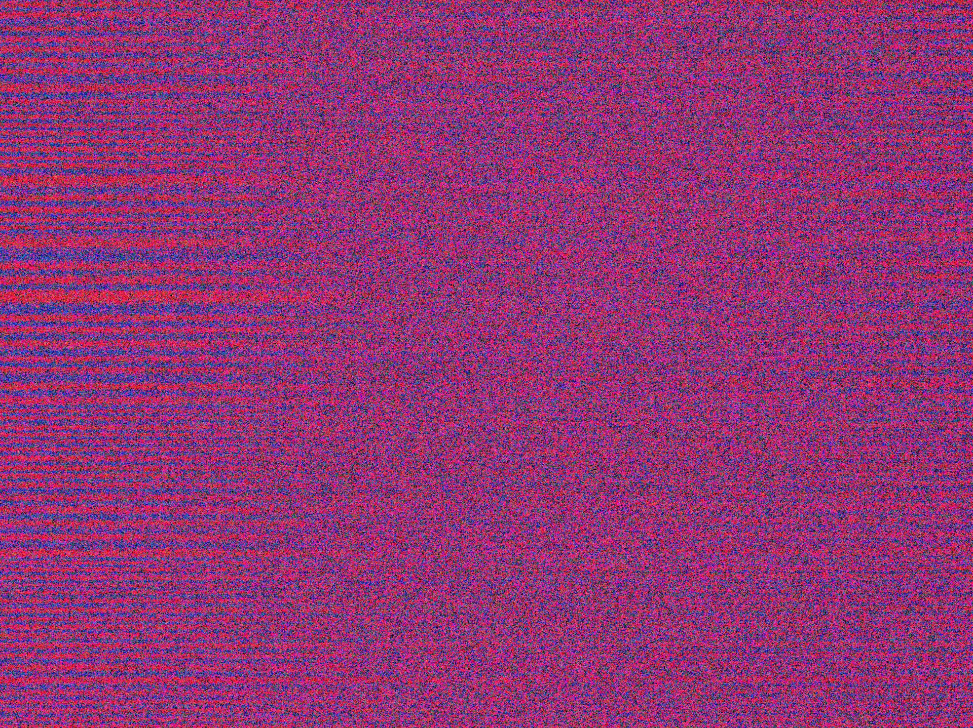
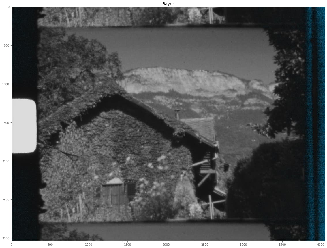
So let’s start with the raw Bayer image of the sensor. This looks like this:
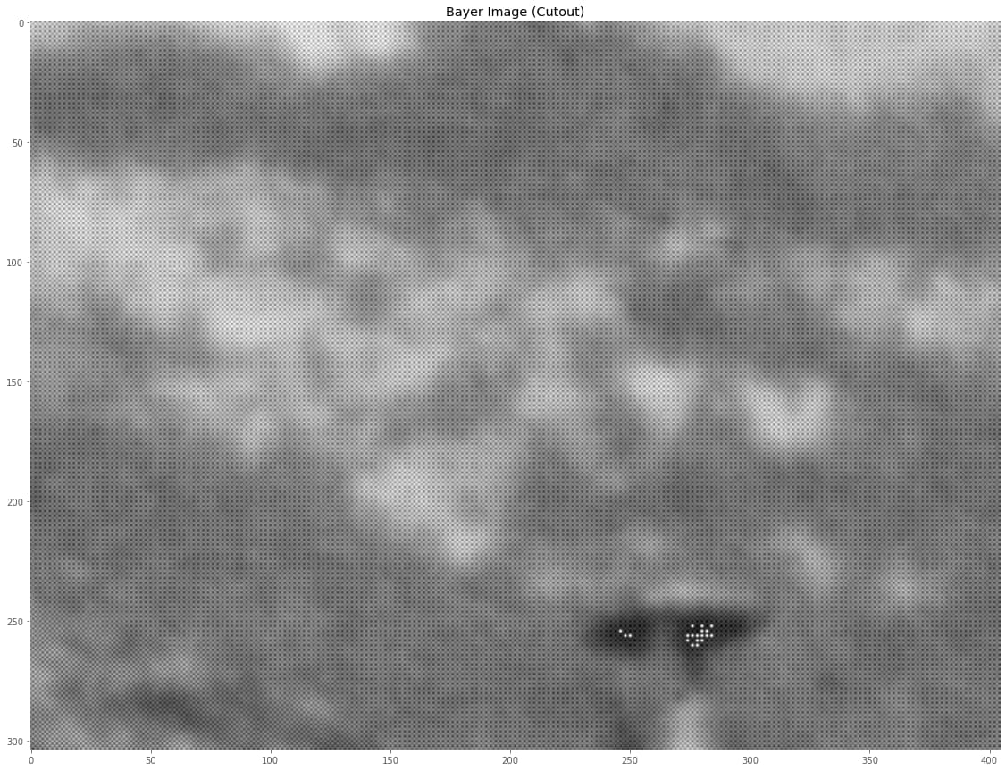
This is in fact a monochrome image with 4 different color channels intermixed. A zoomed-in cutout of the center
shows this interleaving.
Note in the above full view of the capture the appearance of cyan areas on the right side of the raw Bayer image. In all of the displays in this post, very low values will be marked by a cyan color, very high values with a red color. The cyan areas at the right side of the Bayer image are already an indication of the noise floor of the sensor - of course, drastically enhanced. Under normal circumstances, this would not be visible.
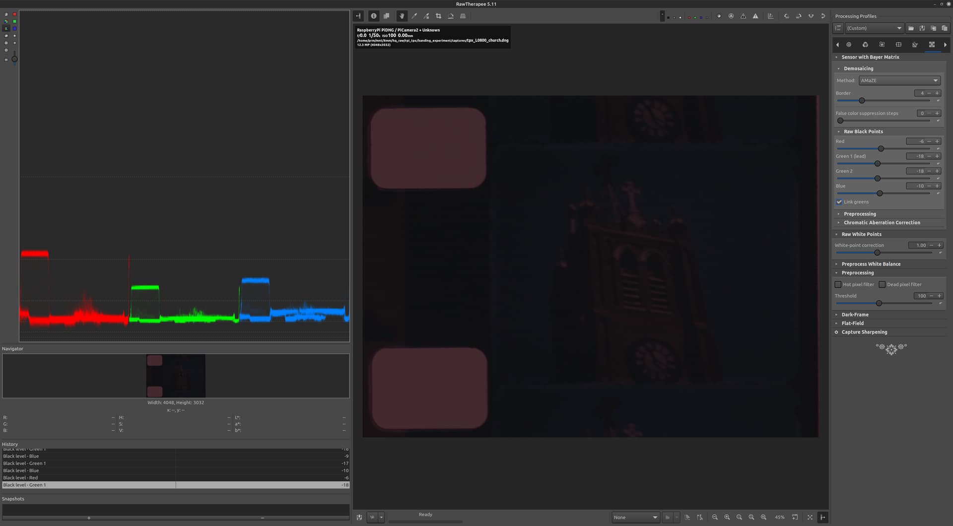
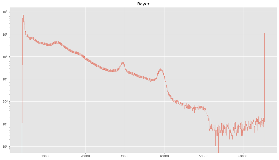
The histogram of the Bayer image looks like this:
The data ranges cover nearly all of the available range between blacklevel and whitelevel. Specifically, we find
Black:      4096.0
White:      65535
Min Bayer:  3920
Max Bayer:  65520
So - the maximal pixel value stays below the whitelevel - therefore, no red markers in the above image, but the minimal pixel values go below the blacklevel - check the cyan areas on the left.
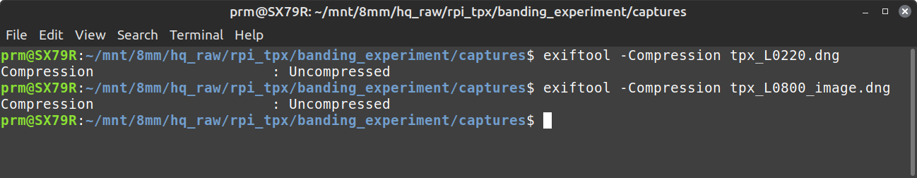
Of course, that should actually not really happening - but in contrast to more advanced approaches, libcamera/picamera2 does not measure the current blacklevel of the camera, but inserts into the .dng just a fixed number. The blacklevel of a sensor is however a function of a variety of things, including sensor temperature etc. Well, …
The histogram of the Bayer image is not so easy to interpret, especially because it mixes the histogram of 4 different channels into a single histogram. So the next step is to create three color channels, here termed “Raw RGB” out of the Bayer image.
Usually, this is done by rather elaborate demosaicing/debayering algorithms. In this demonstration, I stick with the simplest one: just sub-sampling the different channels into four separate channels designated red, green1, green2 and blue, and finally combining them into a single RGB image like so:
camera_raw_RGB = np.dstack( [red,(green1+green2)/2,blue] )
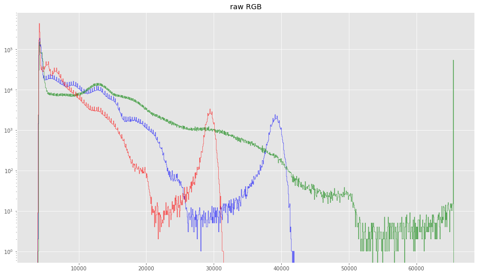
If we look now at the histogram of camera_raw_RGB, we obtain this:
That looks nice. The red and blue histograms are similar in shape, the green one is stretched out a little bit too far, so it’s missing (cutting off) the bump visible at
30000 in the red and
40000 in the blue channel. These bumps correspond in fact to the intensities of the sprocket hole, the brightest area of the image.
Generically, looking at the green curve, the real image content of the frame is distributed from slightly below 4095 up to around 50000. The histogram part of the green channel between about 50000 and the cut-off comes actually from the border of the sprocket area. Since the red and green channels are lower in intensity, the bright sprocket hole shows up in these histograms as broad bump, this bump is missing in the green channel, it is cut off here.
In fact, all histograms are similar in shape, only stretched out differently. This is a direct result of the chosen illumination source. In our case, a whitelight LED with a cct of about 3200 K. If I would have used a different light source, the stretch-factors between the different color channels would be different.
Now, the characteristics of the light source obviously have to be accounted for. This is usually done in a rather simplistic way, by specifying a correlated color temperature for the light source, or, in our libcamera/picamera2 context, by specifying the red and blue channel gains. The inverse of the gains are encoded in the As Shoot Neutral-tag of the .dng.
But before we account for the characteristics of our light source, at this point in the processing scheme, another operation is asked for. The reason is the following: if we would continue with this image data directly, we would finally end up with a noticeable magenta tint in highlights of the final image (I skip the details here, see here for a discussion).
We might call this step our “highlight recovery” step. In our case, it’s simply a clipping of the red and blue color channels using the white point data of the light source available in the .dng.
With Whitepoint = [ 2.8900001, 1.0, 2.09990001] (actually the color gains at the time of capture), he actual code doing this looks like this:
camera_raw_RGB_normalized = np.clip( ( camera_raw_RGB - blacklevel ) / (whitelevel-blacklevel), 0.0, 1.0/whitePoint )
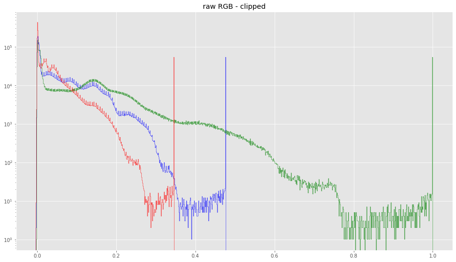
Note that also a rescaling of the image intensities into the [0.0,1.0]range is performed in this processing step. The histogram now changes to this:
The data corresponding to the sprocket hole has now been clipped all channels. All histograms are now looking similar, only the stretch factors are not yet handled. We soon will do this.
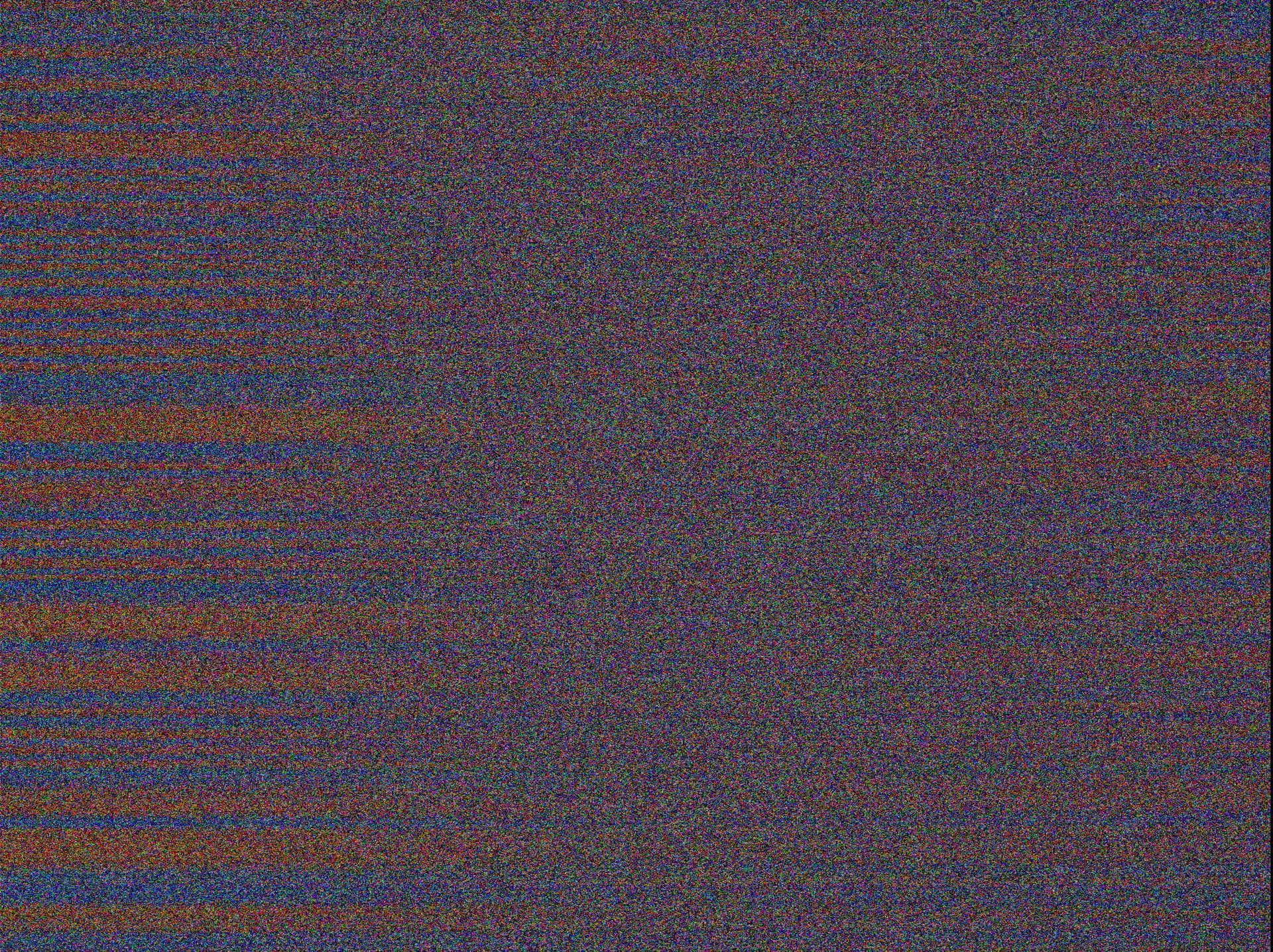
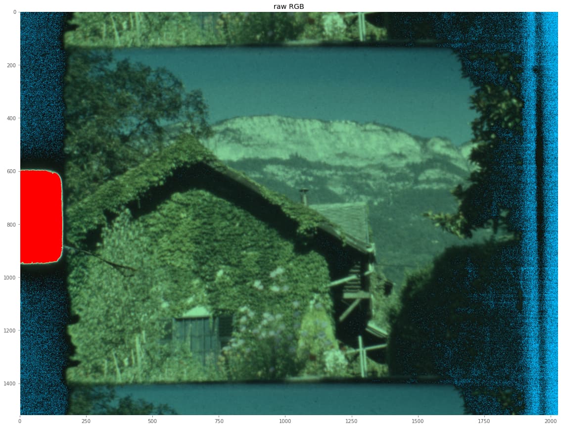
The image resulting from this clipping/rescaling process looks now like this:
Again, pixel values near the noisefloor are marked by cyan, pixel values near the maximal intensity are marked in red.
The noise floor in the above image is now more visible. That is mainly caused by my primitive debayer-algorithm (only sub-sampling). Now the sprocket hole is marked as critically close to the maximum brightness (red colors), and that is ok. We do not want to use the data in the sprocket hole at all.
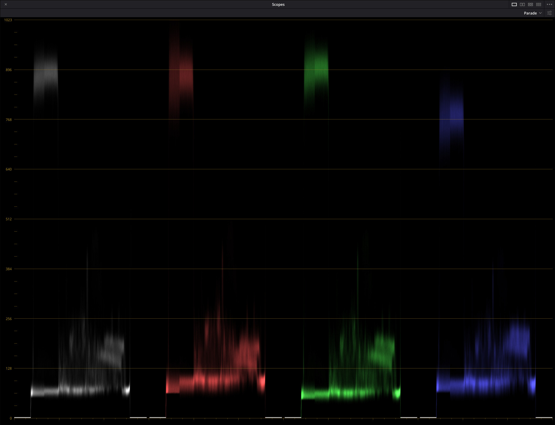
This raw image has the typical green tint of any raw image on the planet and it is now time to convert this into something closer to reality. That is, we must now counteract the illumination still present in the data. As already noted, this is achieved by multiplying the red and blue color channels with the appropriate color gains. The histogram changes drastically
And through that miracle, the curves of all channels magically align. That is just what we are after!
Let’s look at the resulting image:
That looks quite natural, but strictly speaking, the colors are all wrong. Most obviously, the saturation is way too low. To arrive at correct colors, we need to do yet a final step: apply a compromise color matrix to this data.
As per definition, your .dng-file comes with exactly that matrix. Basically, the final computation is something like
img = scene @ camRGB_to_sRGB.T
where the camRGB_to_sRGB depends on the matrix encoded in the .dng-file.
This matrix itself was computed at the time of capture by libcamera/picamera2, based on the red and blue color gains set either manually or automatically. This matrix depends on the correlated color temperature of your light source and shifts the colors finally into their right place.
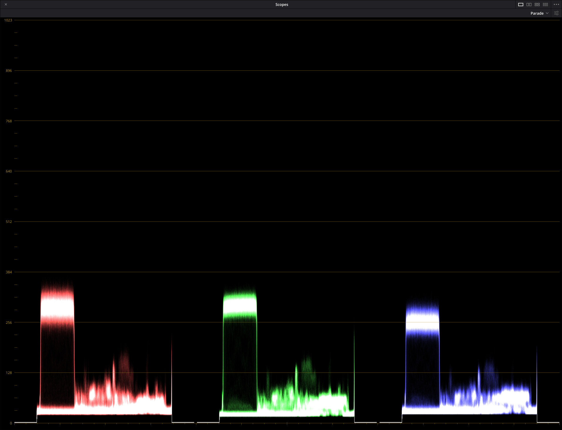
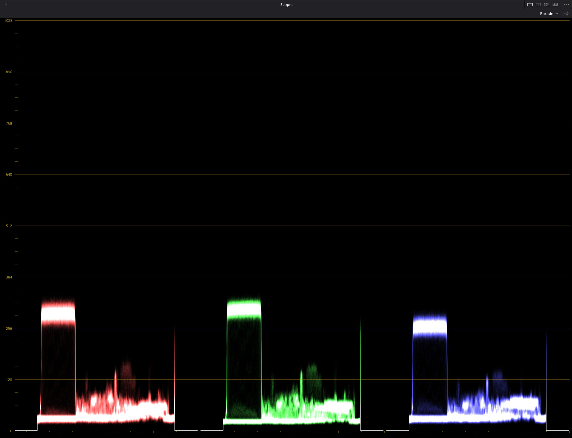
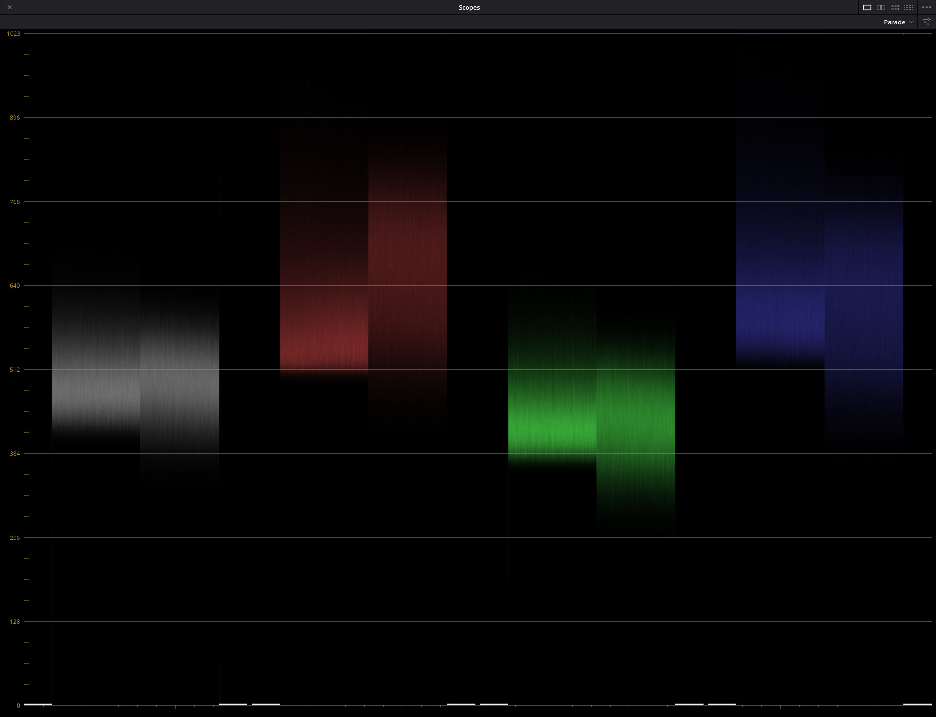
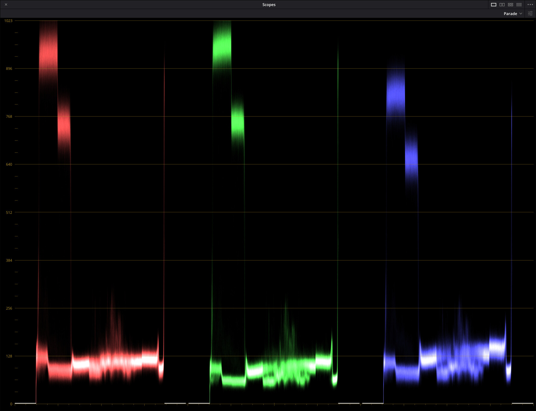
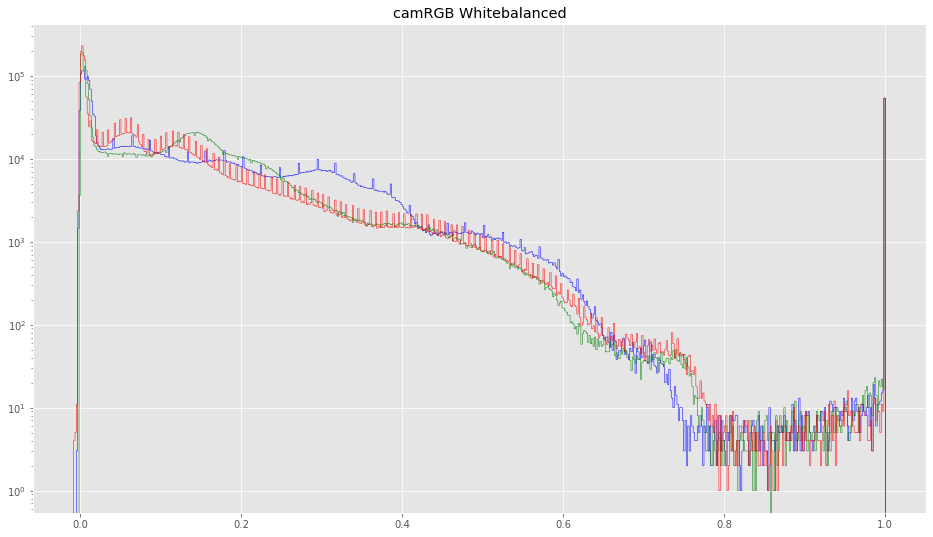
Let’s first check the histogram resulting from that operation:
One thing that can be noticed immediately: there are obviously quite a few pixels in the red channel which are negative. Actually, if you look closely at any of the above histograms, negative pixel values were present all along our way - basically right from the moment when the (not so correct) blacklevel was subtracted from the raw data. Now however, there are much more of these pixels. What are they? Well, that the matrix
camRGB_to_sRGB looks (in this example case) like so:
[[ 1.88077433 -0.83782669 -0.04294764]
 [-0.25912832  1.6064659  -0.34733757]
 [ 0.09087893 -0.74820937  1.65733044]]
There are strong negative components and they shift pixels with original low values in one channel (say: the red channel of a blue sky) easily into the negative range if the colors in other channels (again: the blue sky) are saturated enough. Our camera is able to capture and encode these colors, but our destination color space (in this case rec709) is not able to handle this. The negative pixel values are an indication of out-of-gamut colors (in this case, in the blue sky area).
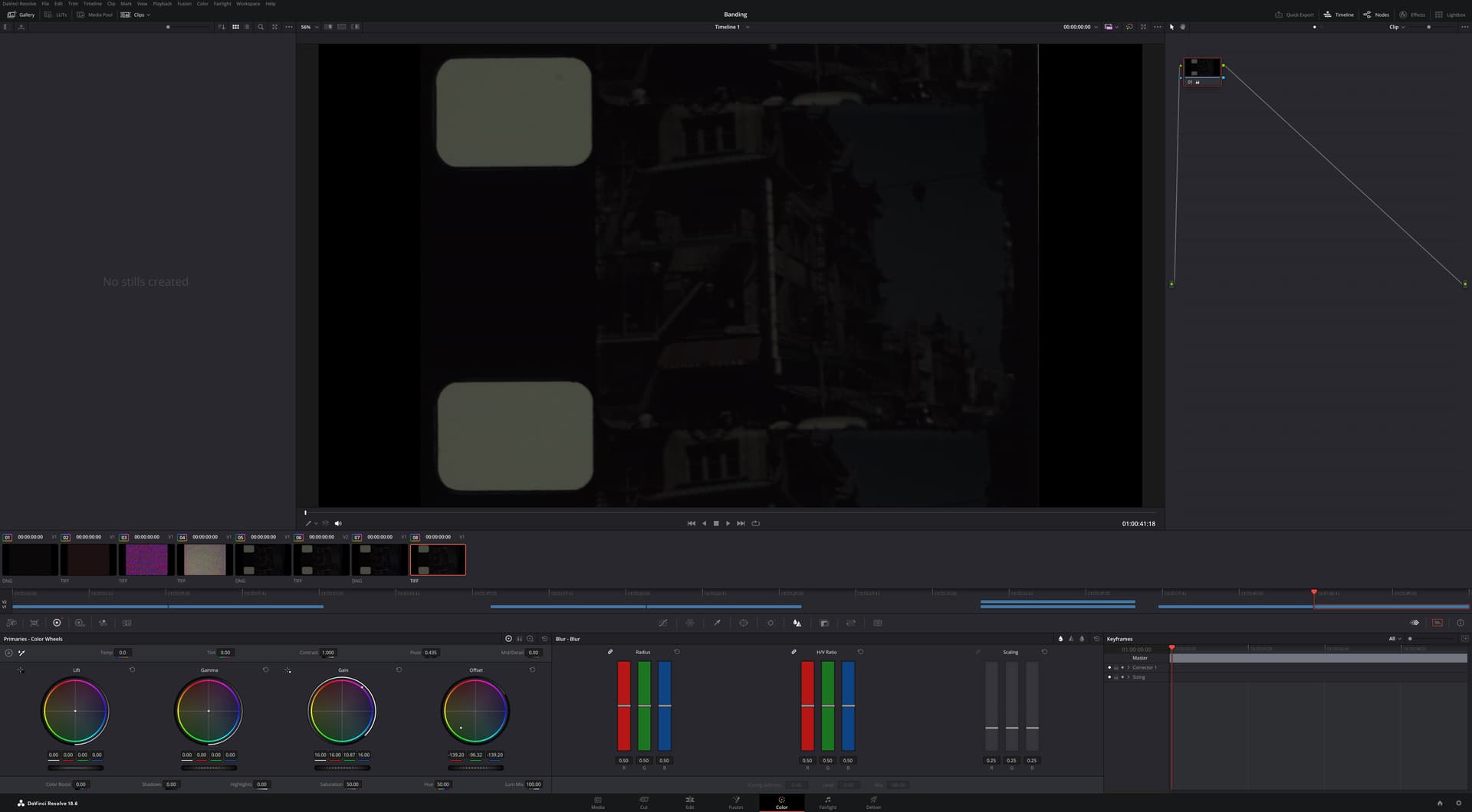
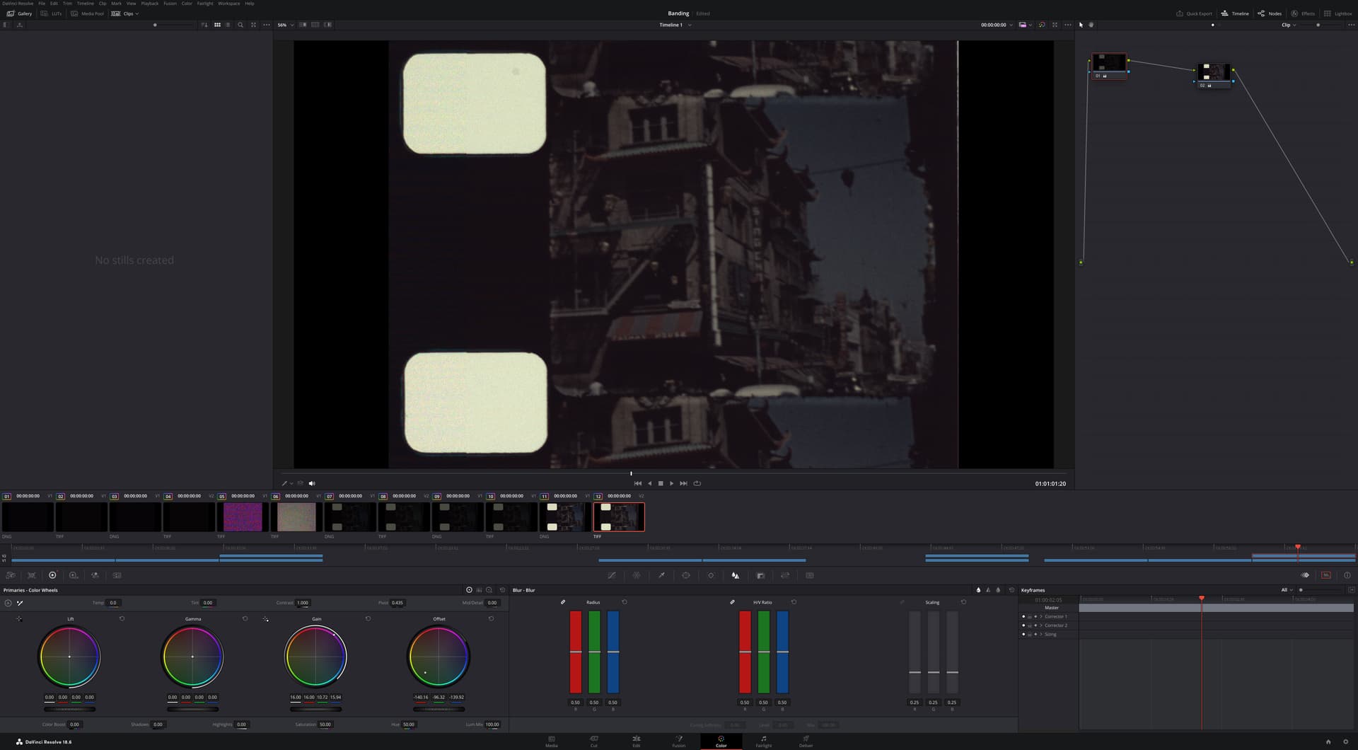
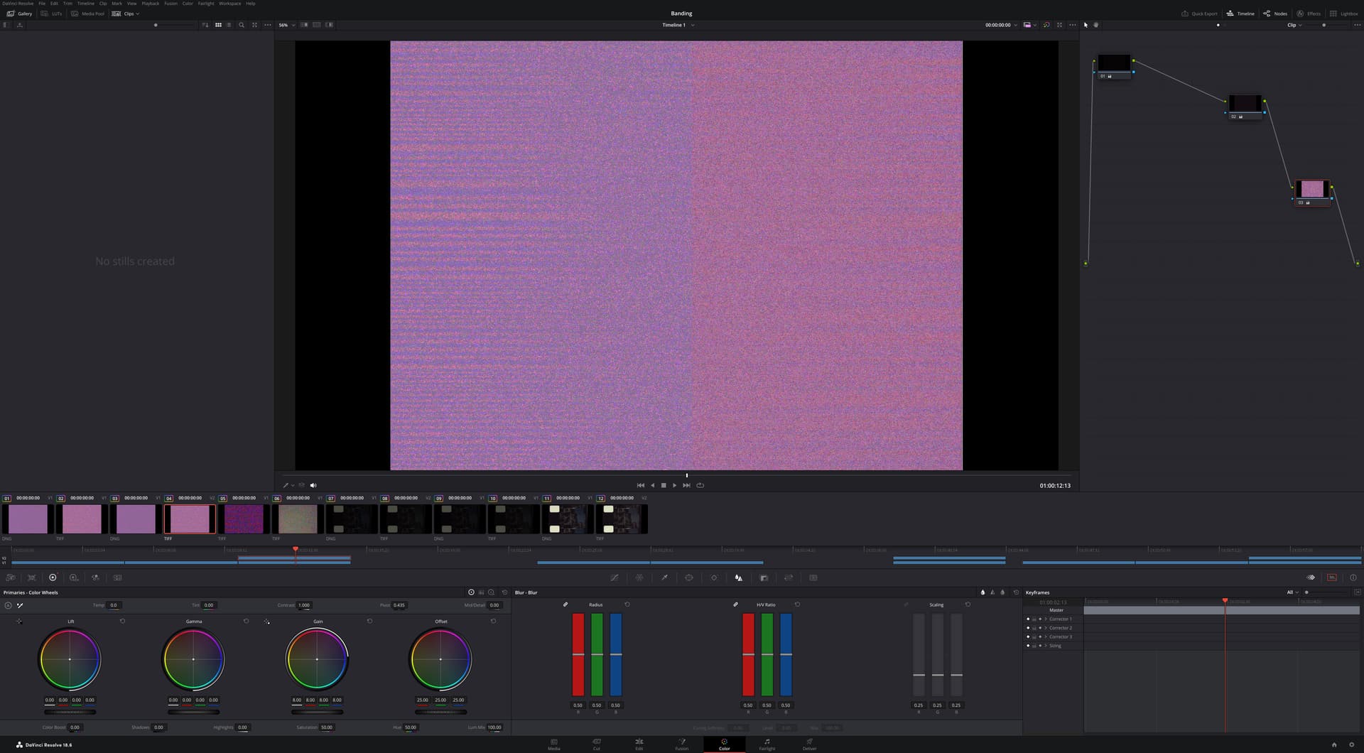
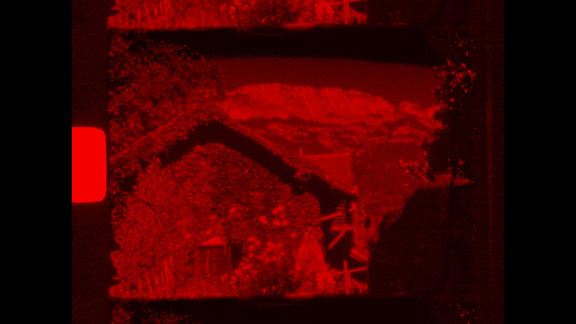
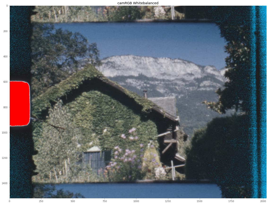
So, let’s look at the final image:
Note that the cyan band appearing now in the sky? This is identical to the black band visible in the red channel above. These pixels have colors which cannot be represented within our current color space. Besides that, note that the low level noise (the noisestripes) has increase as well - the reason here is that the above matrix generally amplifies all color channels a little bit. This makes the noise a little bit stronger.
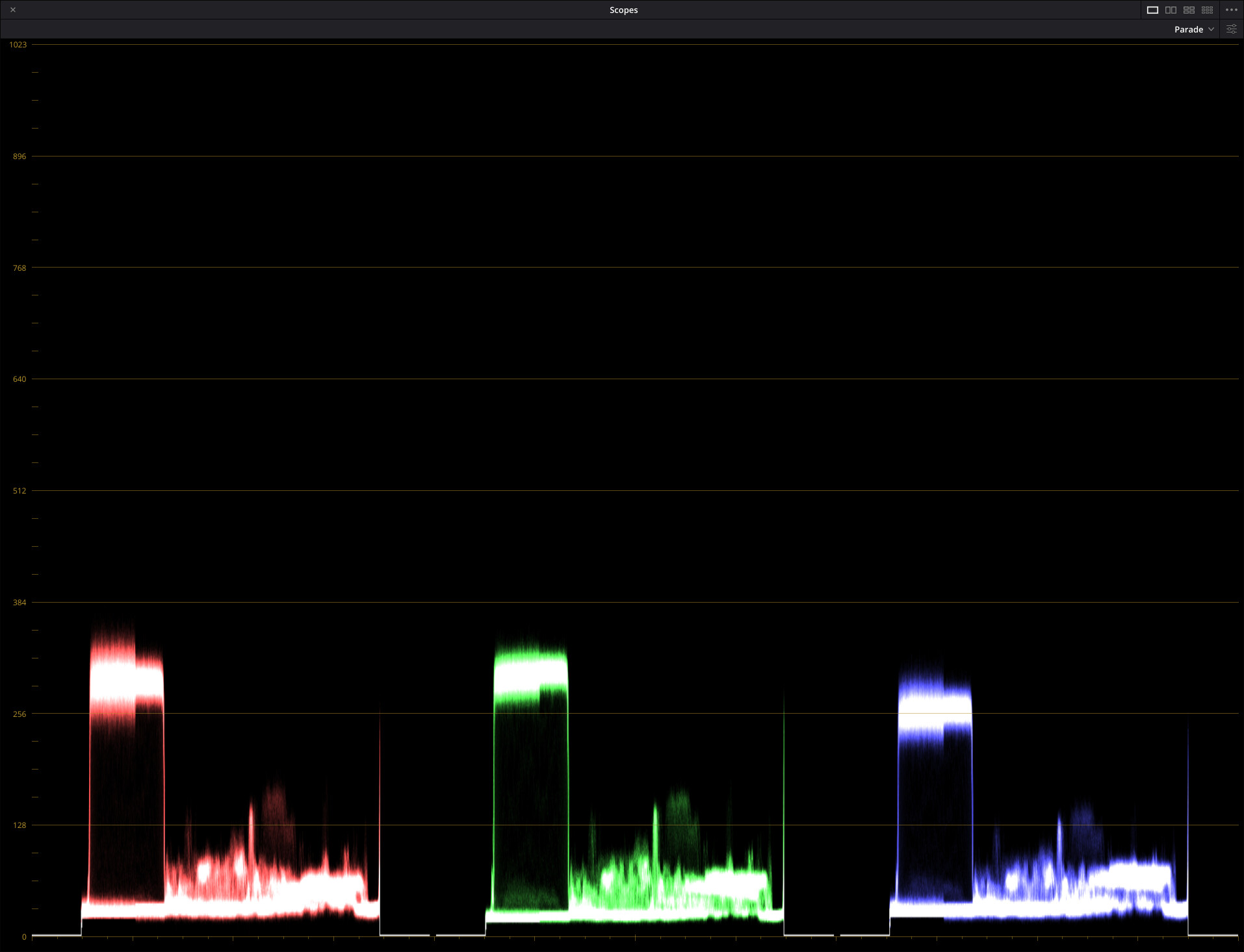
One way to circumvent the appearance of negative pixel values is to instruct the camera to work with a lowered saturation. This would not change the raw data, nor the red and blue gains, but the camRGB_to_sRGB-matrix written into the .dng-file. Clearly, you could ramp up saturation again in your editing program.
Another, better approach would be to map from the start not into sRGB but another, wider color gamut. This would however require a recalculation of the ccm’s contained in the tuning file. Not sure that I am going to go this way.
Yet another option discussed above is pretending that a much wider color-gamut was used while reading the files into DaVinci. This solves again the banding issue, requires again an adjustment of the saturation in post processing. And: - the primaries you are working with are a little bit wrong, so your colors might be off somehow.
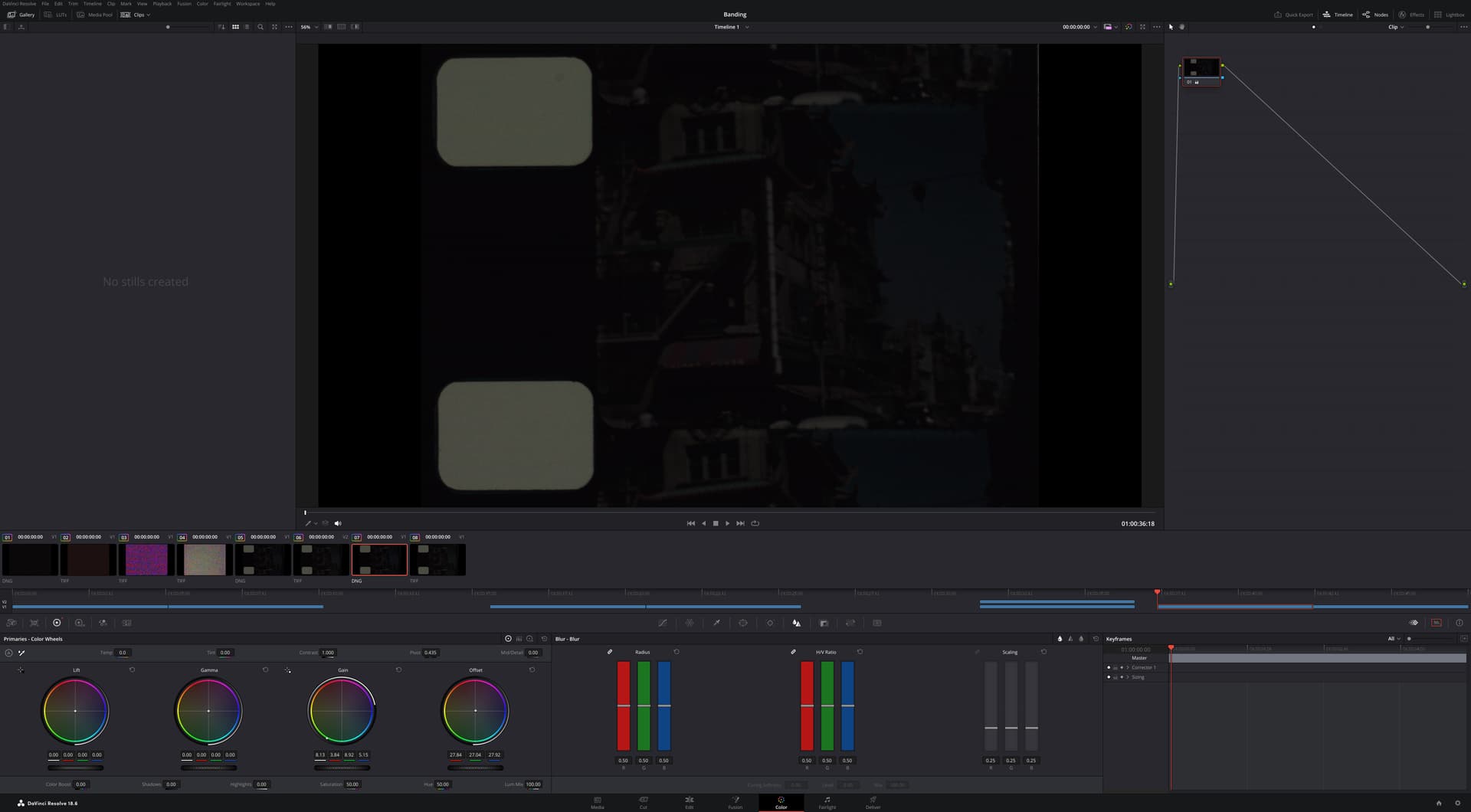
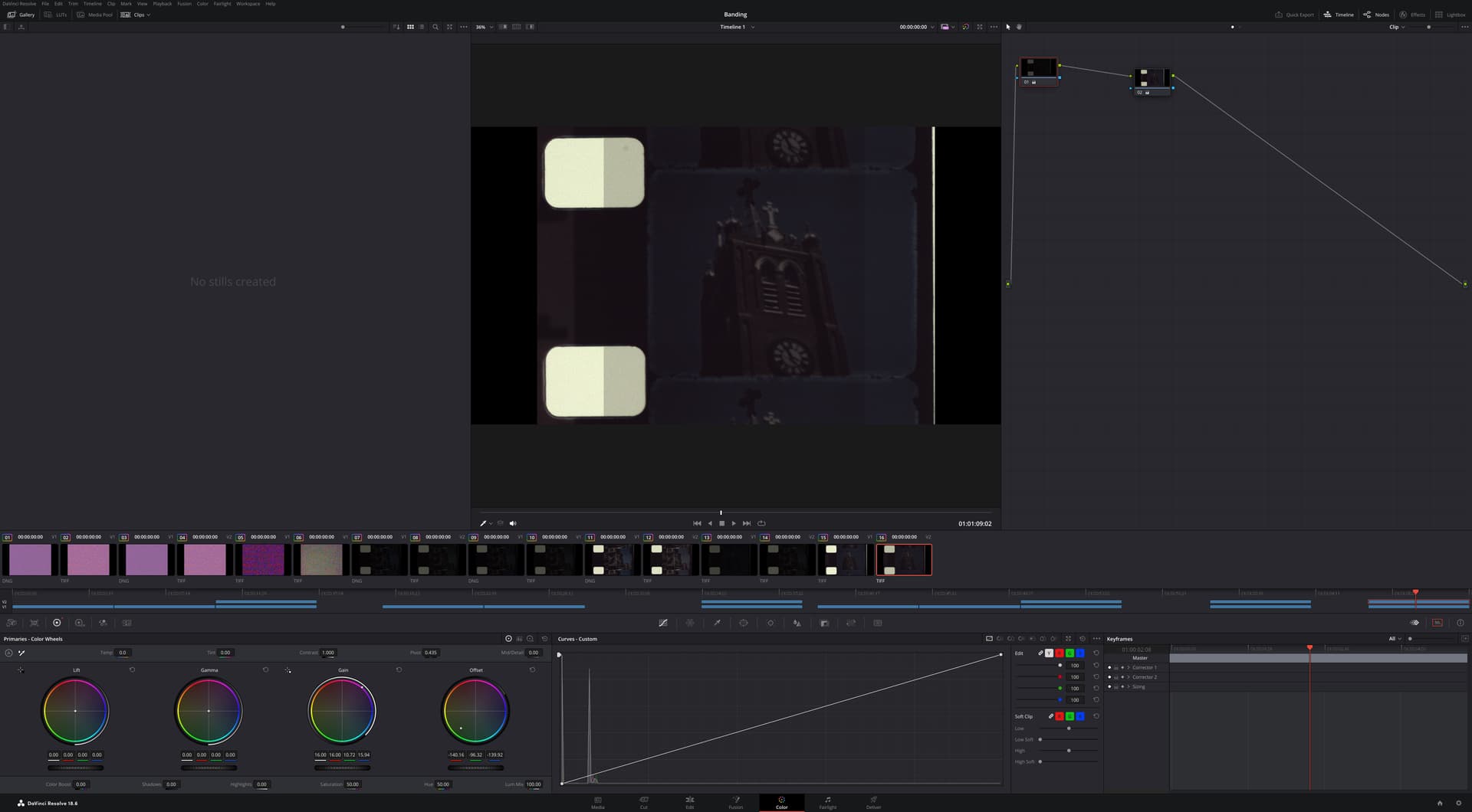
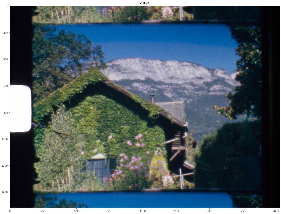
In closing, here’s the above final image without the out-of-limit markings:
I think that is quite usable for a final color grading.