Ok, here’s some quick (but warning! lengthy) examination of the differences between the usual broadband camera filters and narrowband filters. We explicitly do only treat here the case of three independent color channels. Multi-spectral methods usually employ much more channels, utilizing them to get an estimate of the complete spectrum. We will not be concerned with this later use case.
As already pointed out for example by @PM490 (“XYZ sensor”), an ideal camera for photographic use would be one which mimics the filter curves of a human observer as best as possible. Technically, this is not really possible, mainly because the filters one can manufacture are limited in performance. The general approach taken here is to make the filter curves as close as possible, and correct the error with a (possibly scene-adapted) color matrix (ccm) which transforms the camera’s raw RGB values into XYZ values. This matrix is usually the result of an optimization procedure. So, in a sense, every camera sensor combined with the appropriate ccm is actually at least an approximation to @PM490’s ideal “XYZ sensor”.
Now, it’s been some time since I waded through the muddy waters of color science and there might be some error hidden in the following, but I invite you to follow along anyway. The question is: what gives me a lower color error when scanning an arbitrary film frame - a three-channel sensor with broad spectral bands, or a three-channel sensor with three narrow bands?
Since I do not have access to original dye filter curves, but I do have to the spectral distributions of classical color checkers, I recast the intended simulation to a slightly different problem: what performs better, a camera with broad color channels (specifically, I do use the IMX477, the HQ camera sensor, as a test bed) working under standard illumination (D65), or the same camera with the scene illuminated only by three narrow RGB-LEDs. Both situations should be equivalent.
As the test scene, I selected a standard color checker. If this color checker would be viewed by the ideal XYZ sensor, we would obtain the following image:
I now ran three different simulations on this virtual color checker:
- a reference simulation establishing how good the IMX477 sensor is able to record the virtual color checker above when illuminated by standard D65 illumination.
- a first simulation where the color checker is only illuminated by a set of three narrow-band LEDs, with the center frequencies taken from this paper.
- a second simulation where the three LED center frequencies have been tuned manually to improve the residual color error.
All simulations were done the same way: the initial raw camera values were first whitebalanced, so that any neutral patch in the scene (patches 18 to 23 above) has equal amplitudes. Than, an optimized ccm was calculated aiming at mapping the raw camera values to the correct XYZ values the patch colors should have. This mapping, being constrained to matrix, is the limiting factor in the whole processing chain. In any case, the XYZ colors obtained are mapped into sRGB for display purposes and the color error (\Delta E_{ab}) is calculated for the full set of patches.
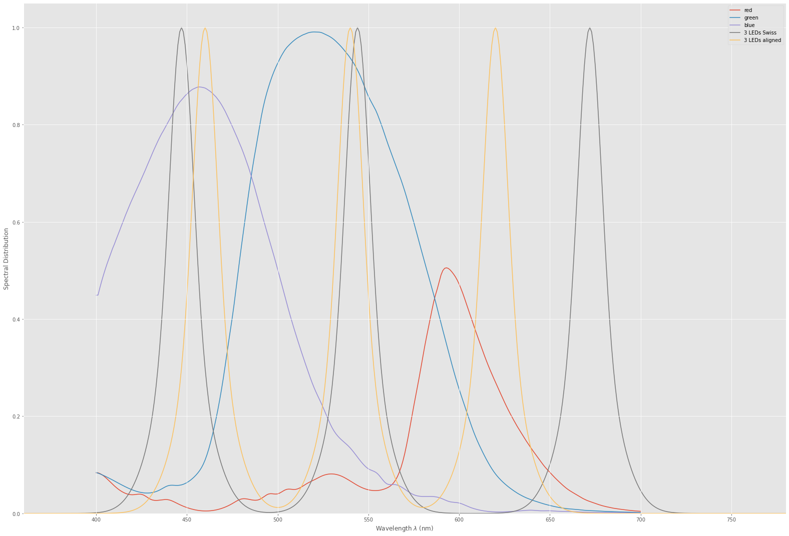
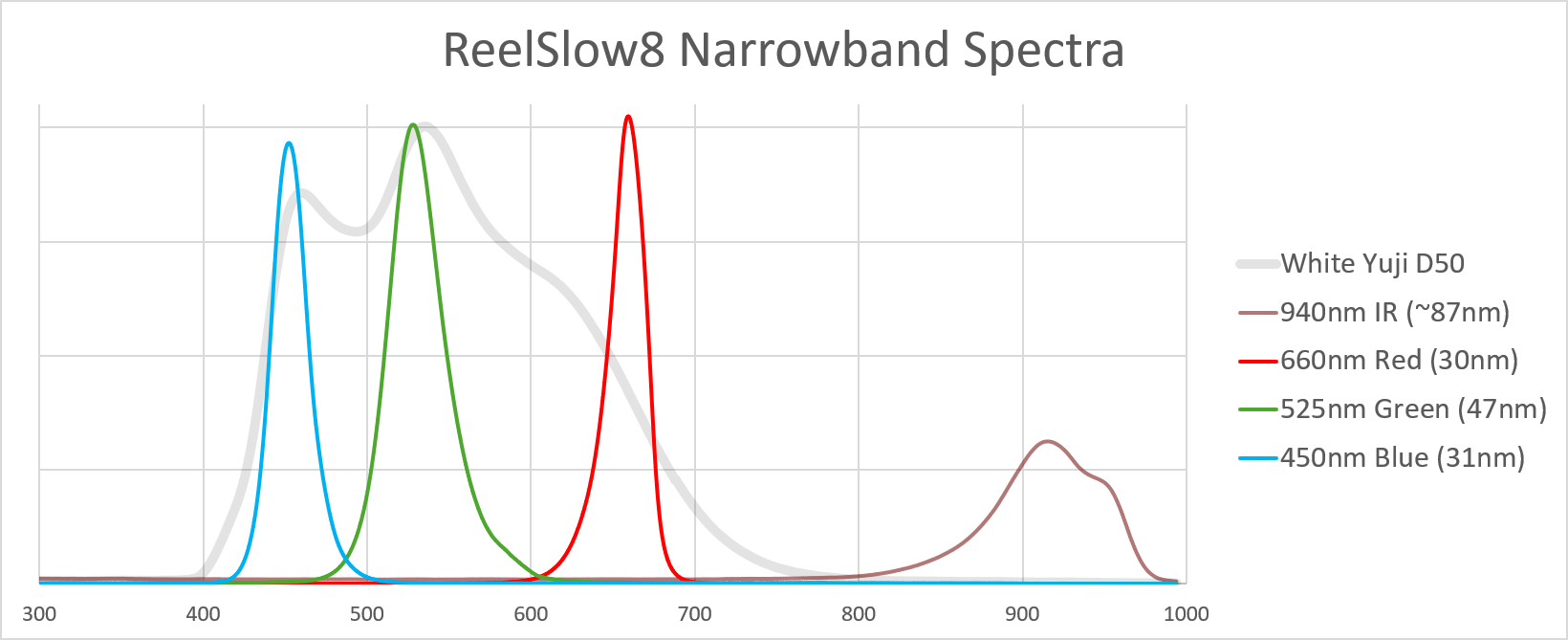
Before continuing to the final result, let’s have a closer look at the sensitivity curves in question.
The curves labeled “red”,“green” and “blue” are the filter curves of the IMX477 sensor with the standard IR-blockfilter of the HQ camera applied. The “3 LEDs Swiss” is the first set of the narrow band LED configuration I have tested. The center frequencies are at 447 nm, 544 nm and 672 nm and were taken directly out of the paper I referenced above. Since I do not have data on the width of a single band, I arbitrarily have chosen this value to be 20 nm for all. Note that while the green LED channel is close to the maximum of the green IMX477 channel, the blue LED channel is shifted towards the UV range in comparison to the IMX477. The shift of the red LED channel is even larger - it ends up in touching the near-IR region. As a result, note further that nearly the whole frequency range of the red channel of the IMX477 is not represented by the “3 LEDs Swiss” setup. The yellow curve in the above diagram (“3 LEDs aligned”) is finally a setup I came up with where I manually tuned the center frequencies of the narrow bands to improve the overall color error.
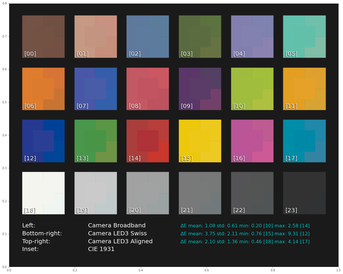
Ok. Now it’s time to have a look at the results. In the following image, the center portion of each patch displays what an ideal observer/camera should see - these are our reference colors. The left half of each patch displays what the IMX477 sensor with its broadband filter curves was able to make out of the data. On the bottom-right of each patch, the reults of the “3 LEDs Swiss” configuration is displayed, and finally, top-right the results of a manually tuned “3 LEDs aligned” setup can be found:
The most interesting numbers on the display are the “\Delta E mean” values. Anything above 2.0 is an error which is deemed to be noticeable by a human observer. So the broadband filters of the IMX477 do perform quite well, with an average error of 1.1. The maximum error occurs at patch 14 (“red”, with a value of 2.6. Overall, this is quite a good performance.
Looking now at the “3 LEDs Swiss” setup, we discover what I already hinted at in this thread: narrow-band filters are no good if you are working with only three channels. Indeed, the mean error ramps up to 3.8! In terms of error measures, the worst performing patch is patch 12 (“blue”), but visually, patch 09 “purple” has also some punch.
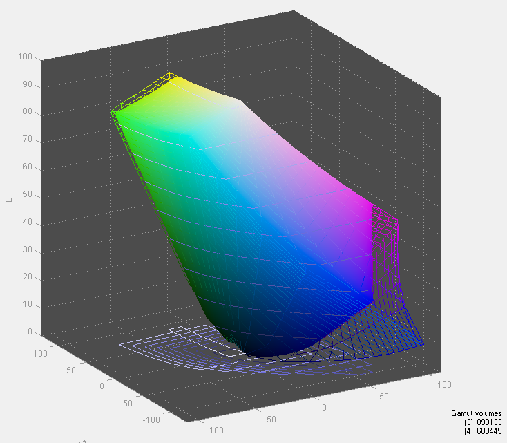
I tried to manually shift a lit bit the center frequencies of the “3 LEDs Swiss” setup in order to improve performance. Especially, I shifted the red channel more towards green, in order to reduce the gap in coverage visible in the above response curve diagrams. This resulted indeed in a reduction of the mean color error from 3.8 down to 2.1. Interestingly, the worst patch turned now out to be patch 17 “cyan” (which is, by the way, out of the color gamut sRGB can display - see plots below).
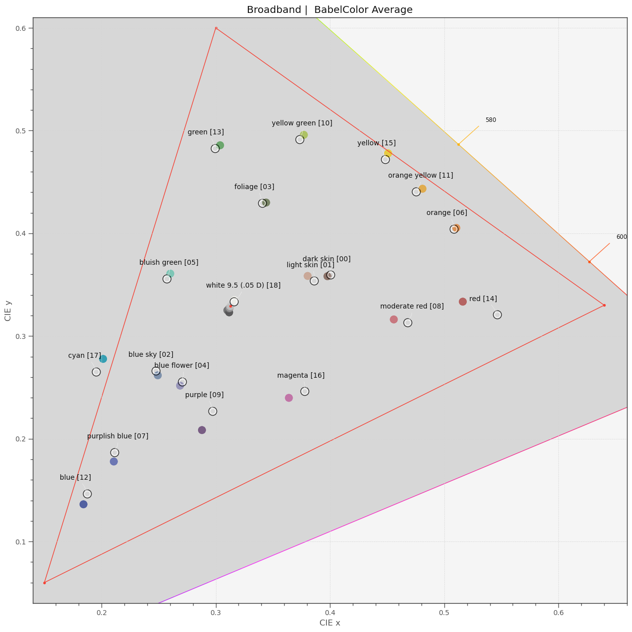
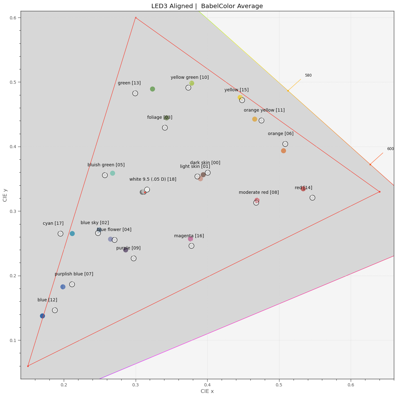
Wrapping up this quick and dirty expedition into color science, here is a plot displaying the colors the IMX477 with its broadband filters came up with in xy-space. The real values are always indicated by black/white circles nearby the color points, the sRGB display space by the red triangle:
This is in fact, as already indicated by the low mean color error above, an excellent performance.
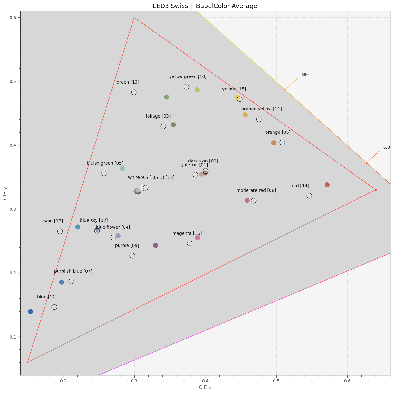
Let’s look at the “3 LEDs Swiss” case:
Clearly, the computed colors do not match the actual colors that well. Especially the colors in the blue and red region suffer.
As mentioned above, I tried to check whether one can do better by adapting the LED’s center frequencies to the material to be scanned. Here’s result of such a manual optimization:
It performs better, especially in the orange-red part. But still, the match of colors is noticeably better when using the broadband filters.
Finalizing this post: again, the results above were obtained by an application of old software I haven’t touched for more than a year. I can not rule out some stupid mistakes. Leaving that aside, I think the above simulations underscore my claim that generally, you are better off by using a whitelight source and classical, broadly tuned camera filters. Here are my main points against a narrowband 3 LED setup:
- with broadband filters, there is a chance of wavelengths falling into ranges were a narrowband system just has dead zones.
- the placement of the centers of narrowband filters influences the achieveable color quality noticeably. The optimal placement probably depends also heavily on the material scanned. If so, the LEDs will need to be adapted/changed once another film stock is scanned. That is impractical in a practical application.
Clearly, if you have anyway a multi-spectral camera with lots of channels (we’ve learned that one should at least consider 8 channels), the impact of the two points noted above gets weaker.