The ReelSlow8 Film Scanner

[npiegdon]

@cpixip

For example, the log-encoding used in some cameras does coarser quantization steps in certain intensity ranges…

I suppose the best part of log encoding is that it roughly matches the sensitivity of the human visual system, so the information that is discarded is the part our eyes are the least likely to miss. (Well, assuming the final, color-graded output exposure is somewhere in the neighborhood of the input. If the footage was incorrectly exposed and needs to be corrected more than a couple stops, even log footage can’t save you from some loss of quality.)

@cpixip

From my experience, it is important to prestabilize the footage before a temporal-degraining operation is attempted.

This is another good point. I’ve already been through a post-processing workflow with a number of home movies from the 80’s and 90’s recorded on VHS tape. In that case, doing motion stabilization before the other cleanup steps did seem to help the final result in the way you described.

[PM490]

@npiegdon

FWIW, last night I ordered some barium sulphate and those small cake pans that @PM490 has mentioned a few times.

Finally got around to make the port holes. Here is how it looks.

Ps. and after a bit of epoxy, here it is with the light ports. I will prototype with prior LCB PCBs.

[npiegdon]

May: Pixel Size, Focus Detection, and Planarity

I didn’t get quite as far as I’d planned on full-fledged auto-focus, but the digression into measuring the size of each pixel was worth it.

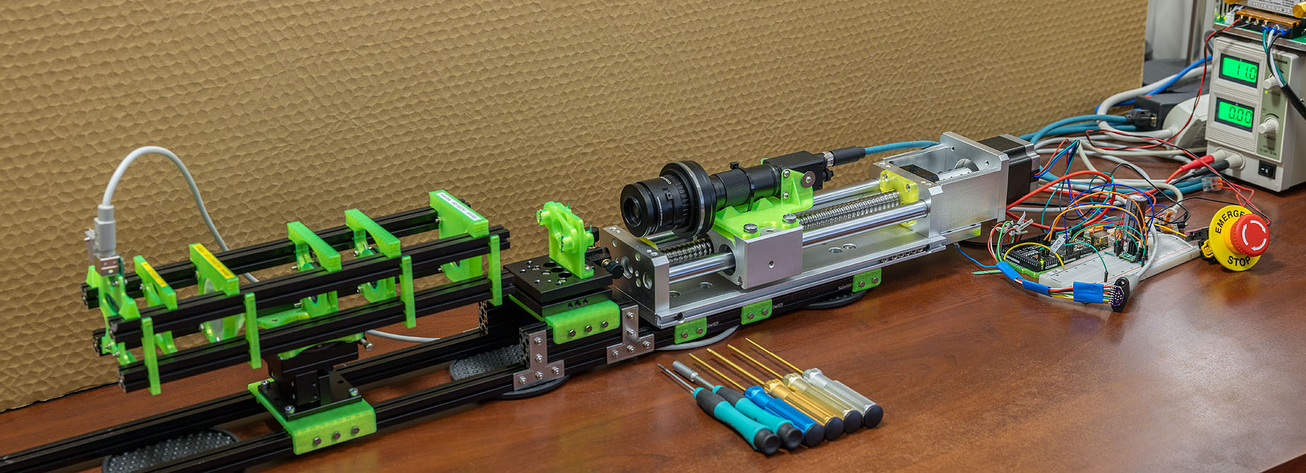
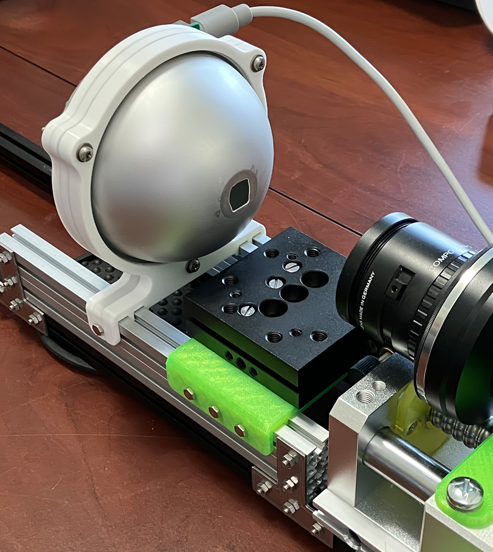
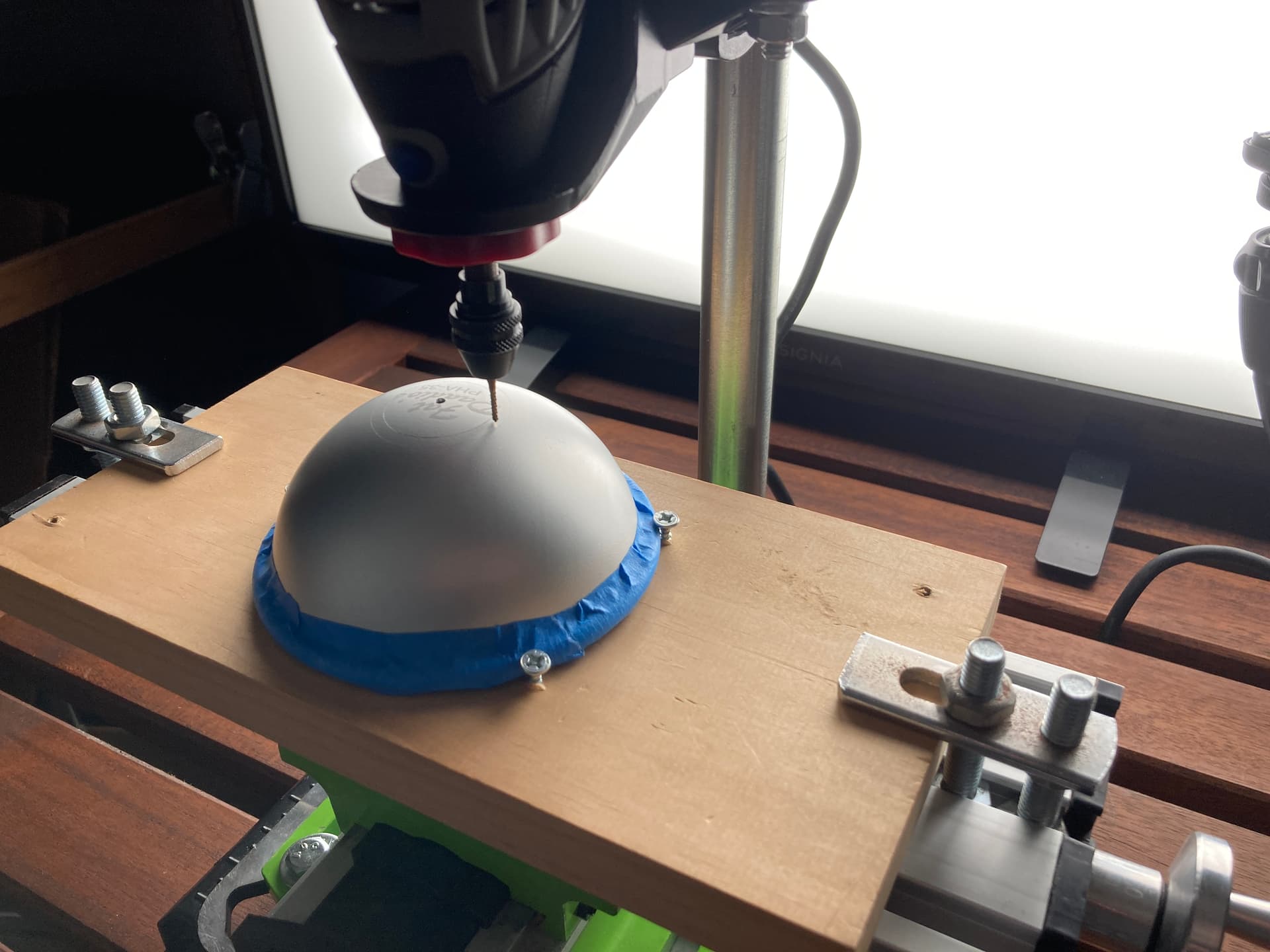
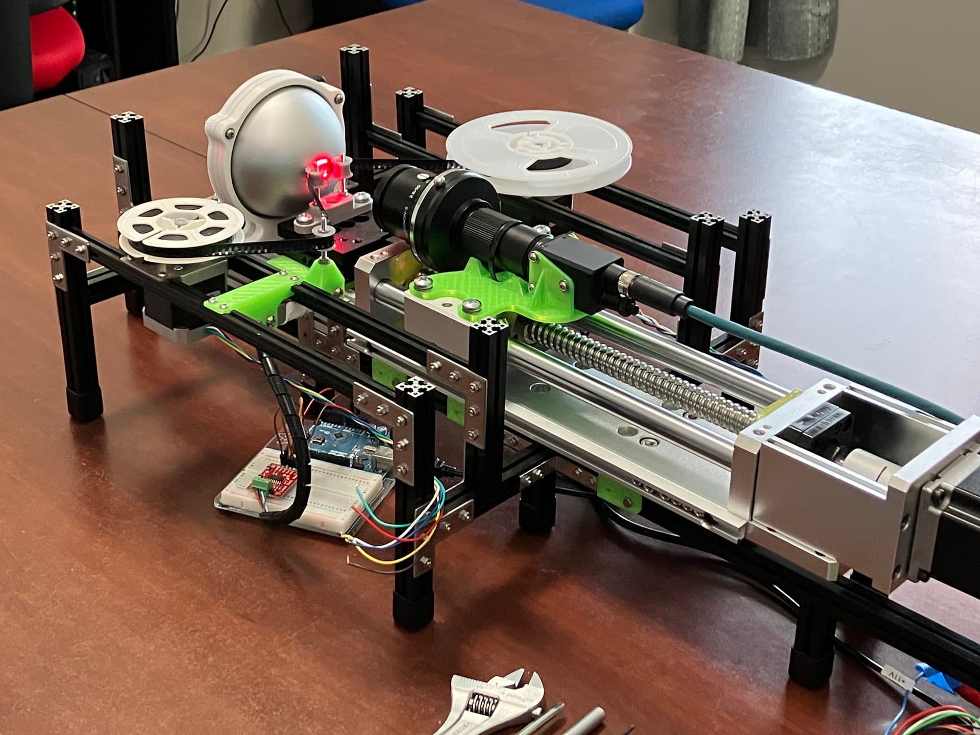
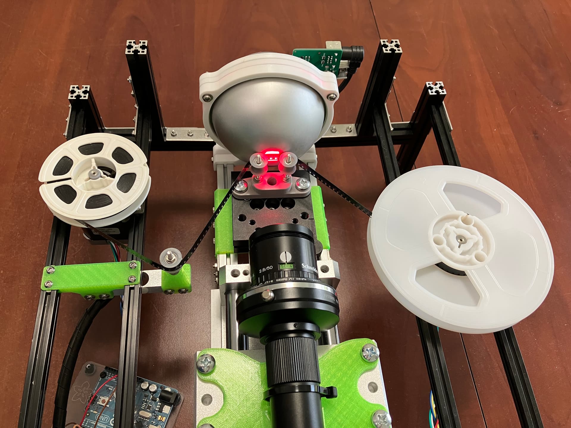
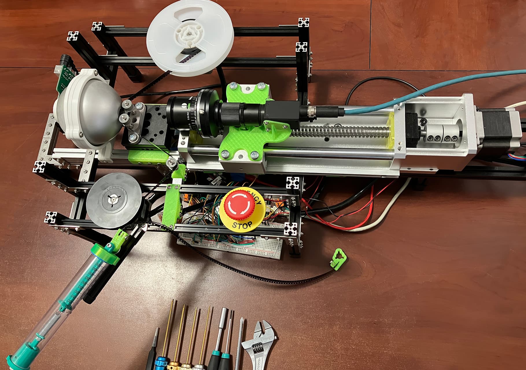
The machine is starting to look like something:

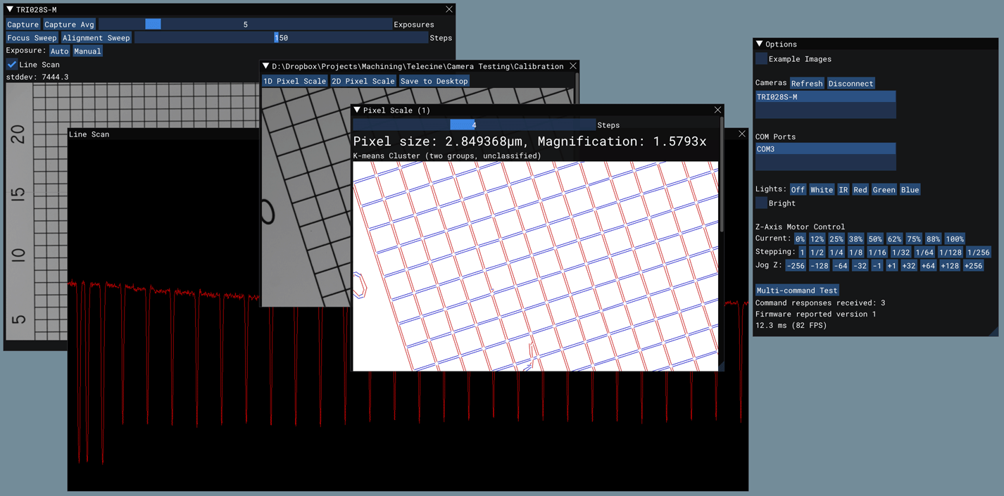
The software is still mostly debug buttons and other manual testing/control bits, but the number of things it can do is steadily increasing:

In particular, I’m happy with my decision to use Dear ImGui for the UI. I’d never used it before, but on average it takes a single line of code to both add a new button and the code for what that button does (no extra callbacks, etc.), so the framework stays completely out of your way and lets you get your work done.

The communication between the Arduino and the Windows app is going smoothly. I came up with a little protocol where each message (and reply) is between 1 and 5 bytes for all of these primitive operations like changing the light color, delaying for some number of microseconds, or taking some number of linear motor steps. But then there is a mode where you can say “start accumulating instructions until I tell you to execute them all at once”. That takes USB jitter, parsing overhead, and most other sources of latency out of the equation. So it should be able to do things like strobe the lights with repeatable timing when triggering the camera’s GPIO pin to acquire an image, if need be.

Measuring Pixel Size

Last time I said my biggest fear was going to be a large change in the size of pixels between the best focus point for each color channel. I’ve since been able to confirm that the size of the pixels does change but not so much that it isn’t something I won’t be able to correct for in software with some very gentle resampling.

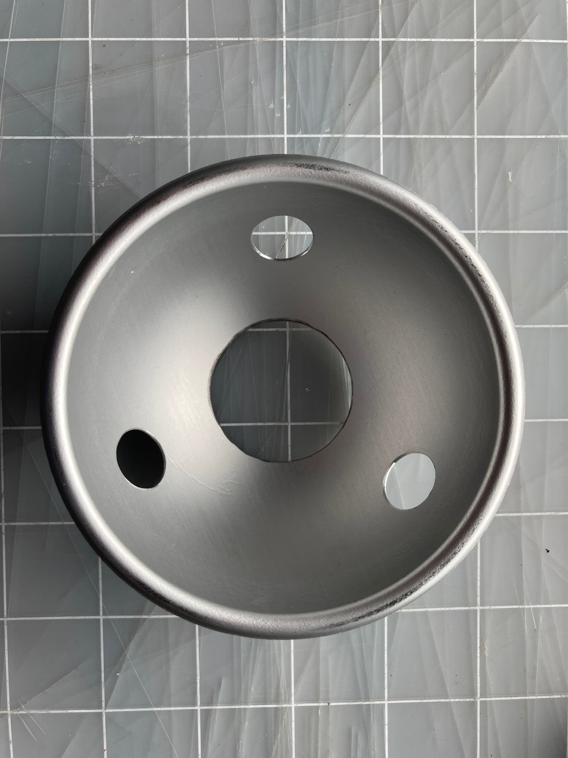
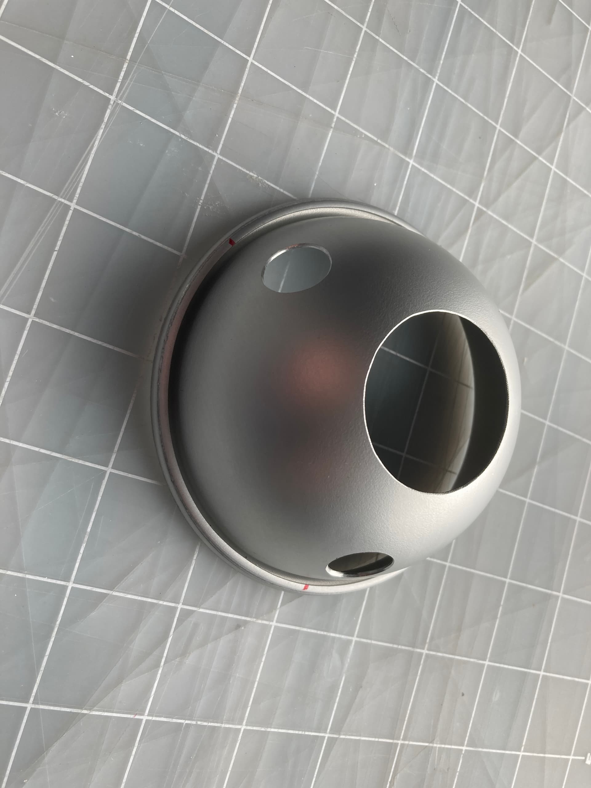
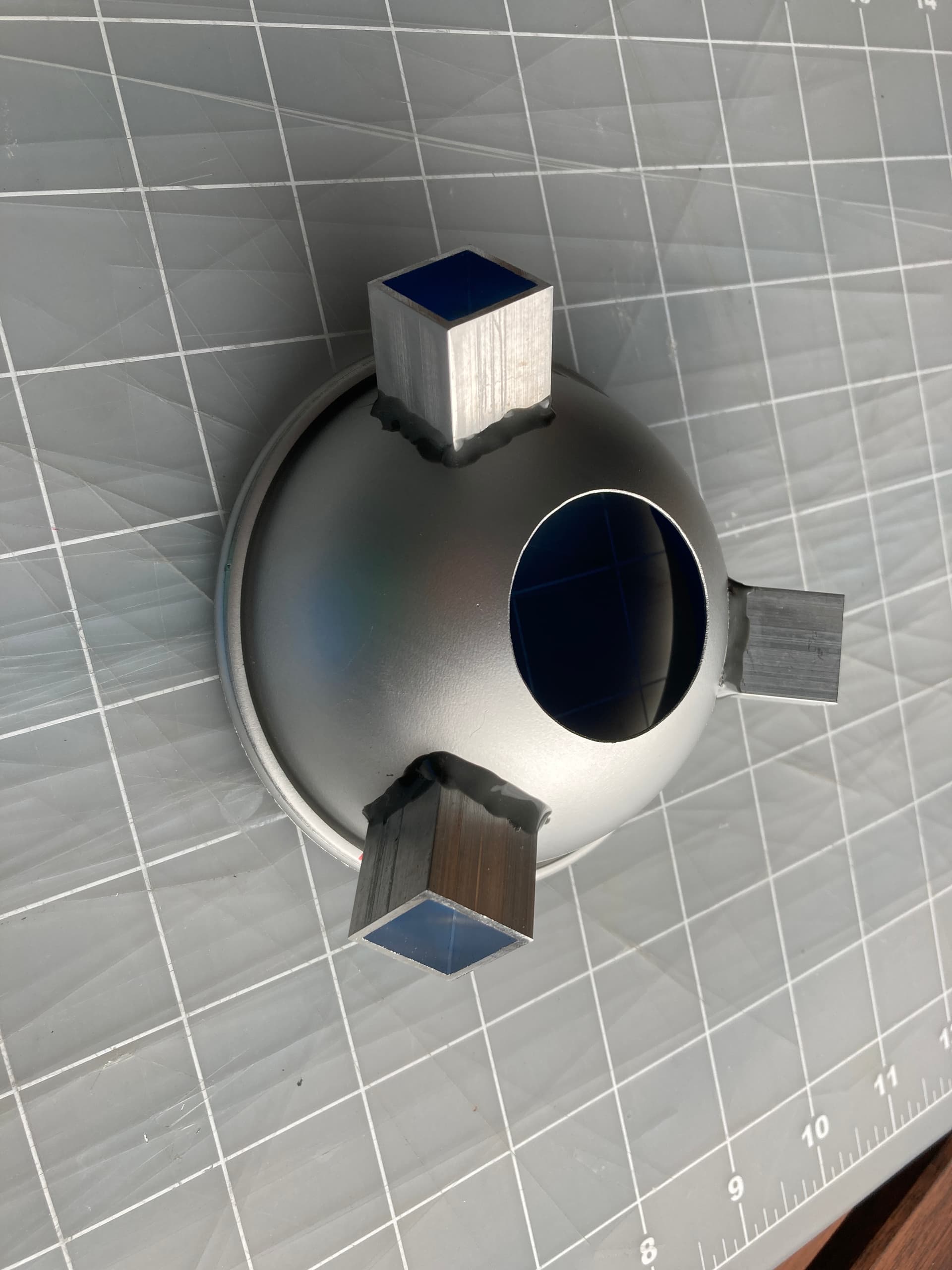
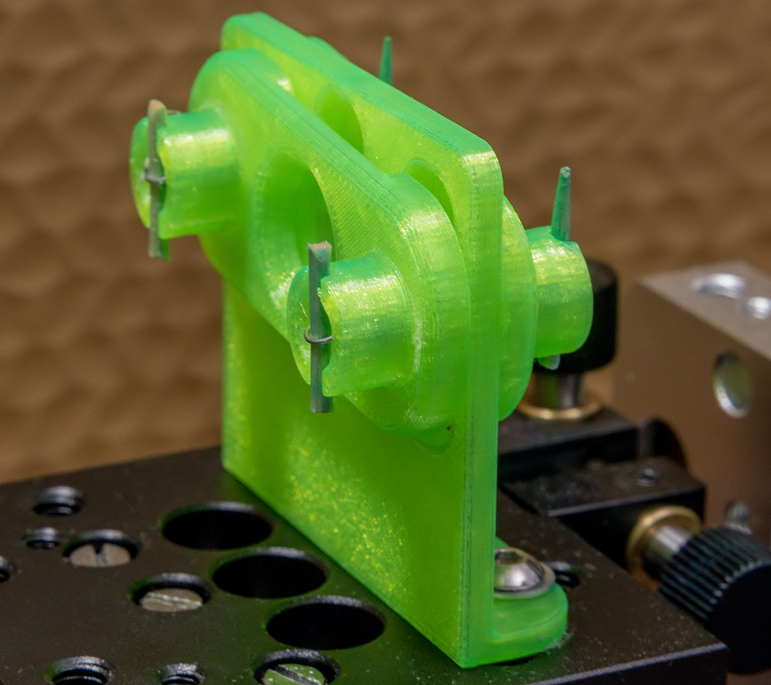
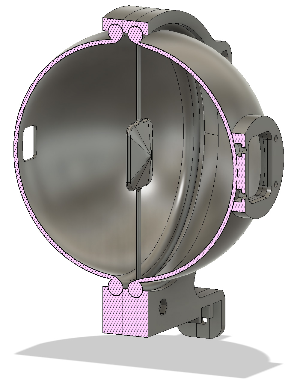
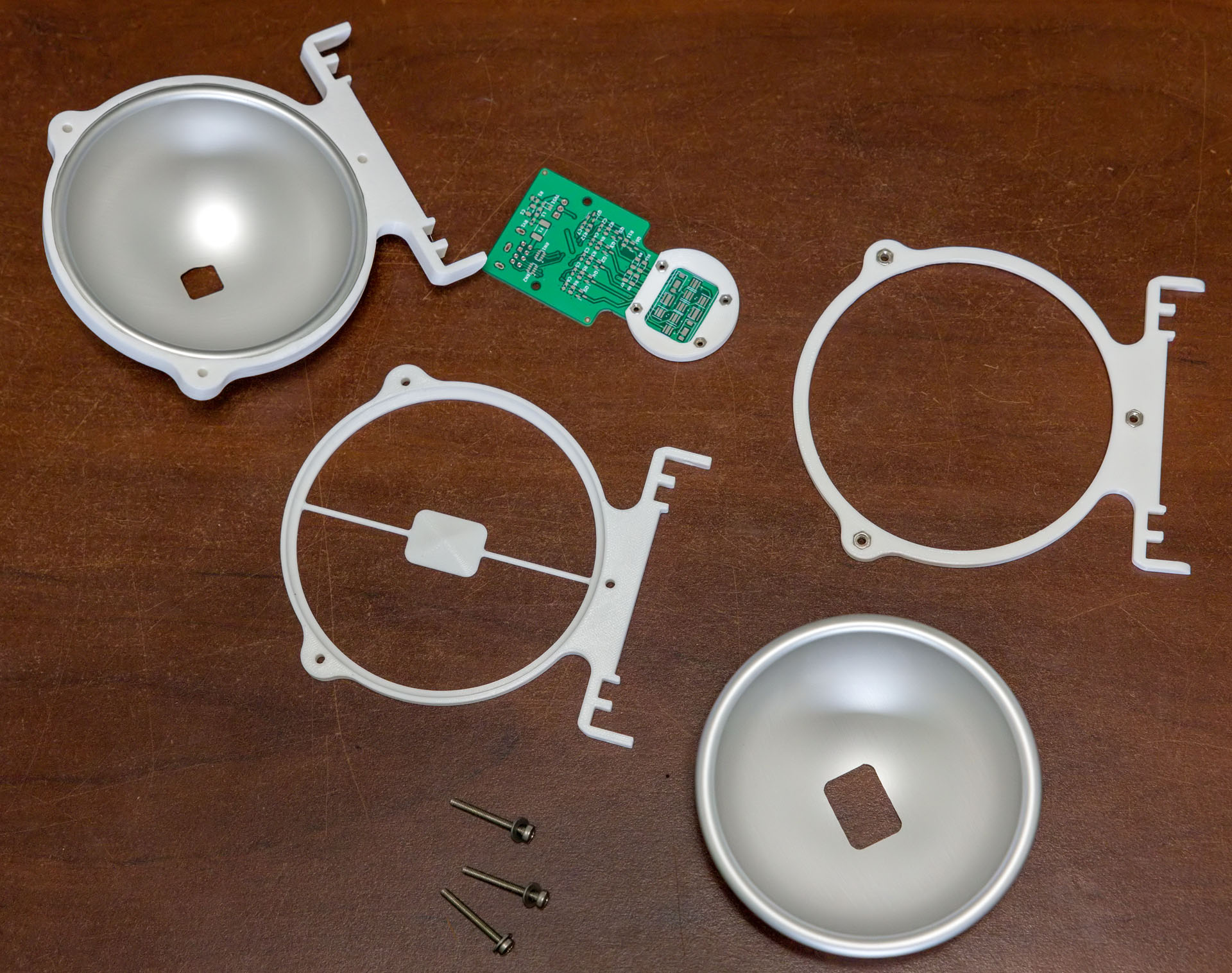
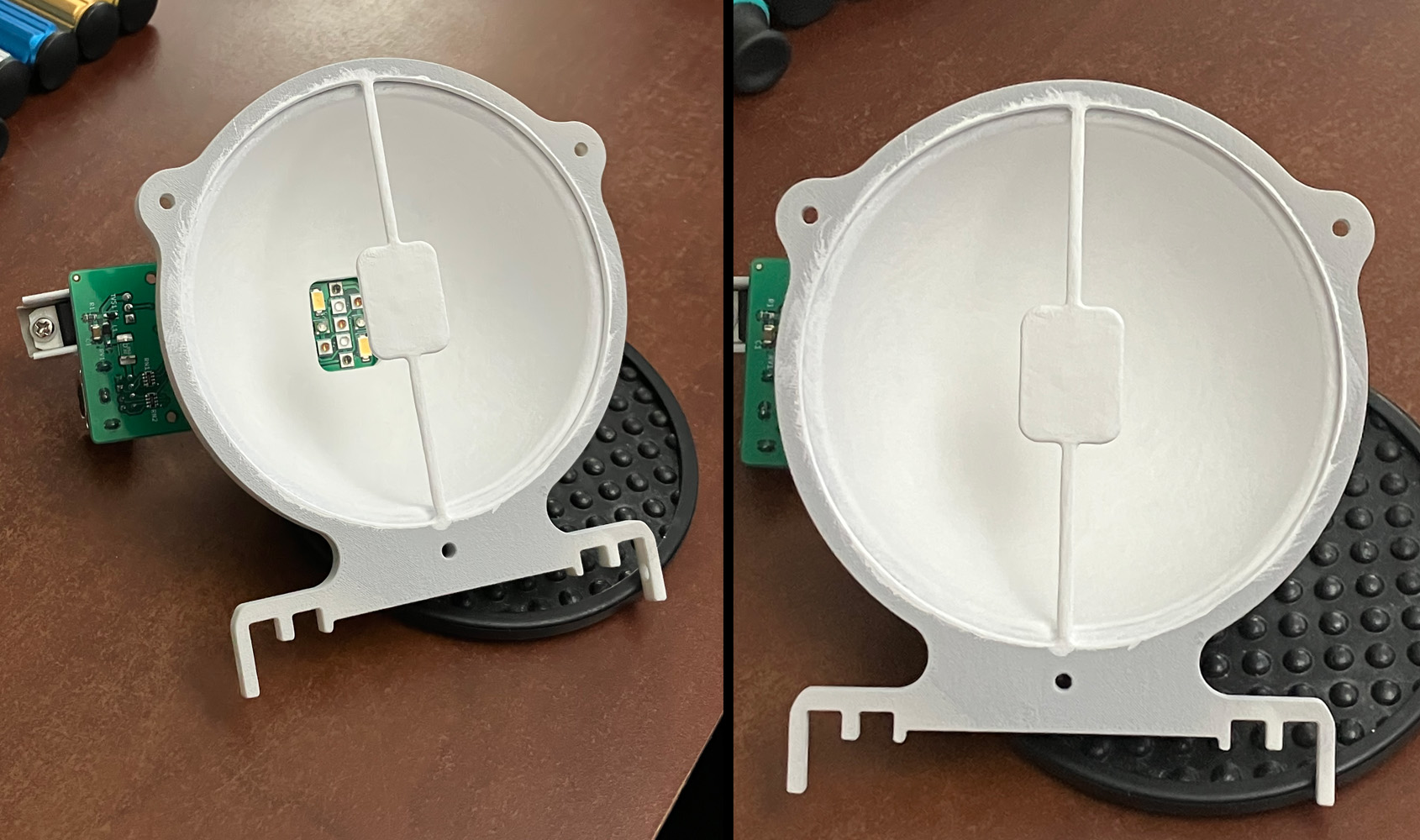
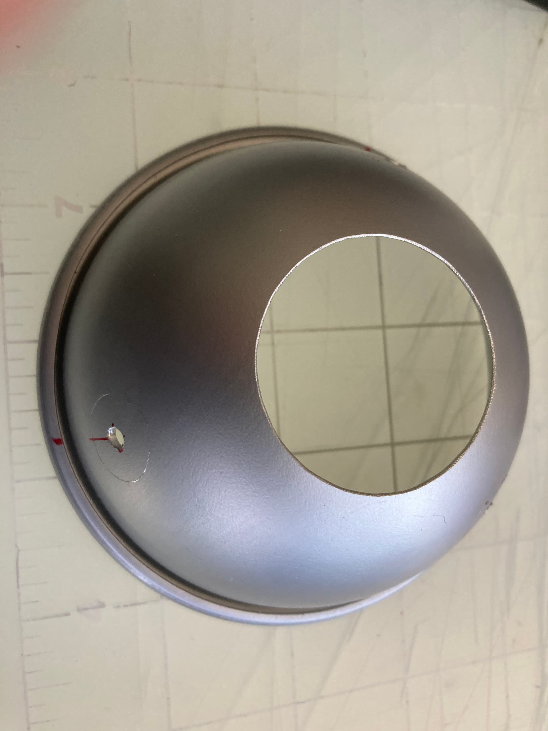
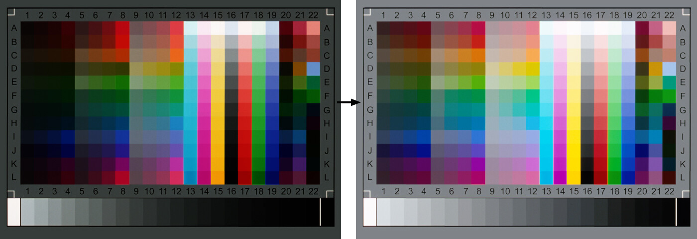
The first step was being able to reliably hold these calibration targets. I was having trouble getting something held in place tightly while still being able to make fine adjustments, so I cobbled together this little slide holder that uses springs to hold the slide against a fixed surface.

Those are toothpicks holding the springs under tension. I switched to a full grid calibration slide that is a small, round disc with a target that’s roughly the size of an S8 frame, which is perfect. So that’s what’s sandwiched between the plastic layers there in the photo.

Until now, I was measuring pixel size manually by capturing an image, using the ruler tool in Photoshop (which snaps to whole pixels), and doing the math by hand. But I wanted sub-pixel accuracy and more measurements to average across to make the result more precise.

After some tinkering with OpenCV, I came up with something pretty cool for the single-axis (1D) target. It was a little brittle and required a nice, sharp capture without any dirt in the frame, but I was getting some reasonably good numbers out of it. But then two days later I figured out how the idea could be extended gracefully to the full 2D grid target in a way that was much less finicky about the quality of the image.

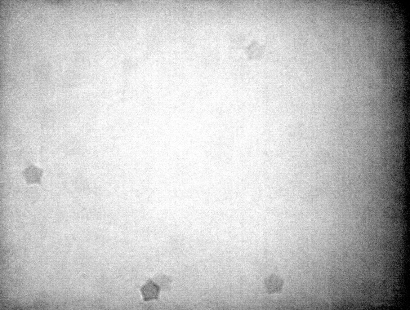
Here are the broad strokes of the algorithm being run on an intentionally skewed and dirty frame to show its resilience:

(Be sure to click the “Play” button on the animated GIF. The forum software seems to prevent it from animating automatically.)

Step 1 is running the CLAHE algorithm built into OpenCV to bump the local contrast up for line detection. There is some gentle blurring being done here too, which I didn’t show in the animation.

Step 2 is picking out line segments using OpenCV’s cv::createLineSegmentDetector. (Specifically this does not(!) use the Hough transform line detection; I spent a lot of time there and was getting poor results, whereas the LineSegmentDetector feature worked beautifully on the first try after I found it.)

Step 3 is where it starts to get cool. Find the angle of each detected line segment (wrapping it into a half-circle so that a 1 degree angle and 359 degree angle show up as 2 degrees apart instead of 358), and then run K-Means Clustering (with two groups) on it. OpenCV also has this feature built-in with a nice, easy API for using it. What you’re left with is two lists of line segments that are grouped by what you might call “horizontal” and “vertical”, except there is no dependency on the grid being aligned with the camera sensor.

Step 4 is now that we have the cluster centroids, which are a kind of “ideal” angle, we can check that they should be almost exactly 90 degrees different from each other, and throw away any line segments that aren’t close. This cleans up almost all of the noise, dirt, and other elements from the image.

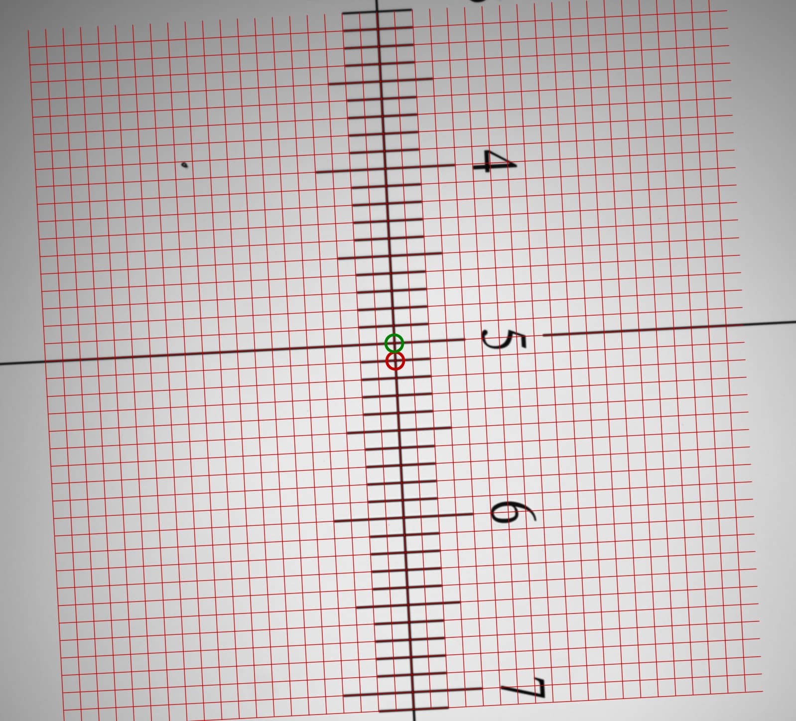
Step 5 breaks each list of line segments into two lists of points containing the end points of each line segment. So, both endpoints from each “horizontal” line go into one big list and both endpoints for each “vertical” line go in a separate list. At this point we are done with the lines and they can be discarded. The endpoints are the blue and red dots in the animation.

Step 6 finds pairs of endpoints–one from each list–that are closest to one another. There is no special ordering required: pick any point from the first list, go through the second while making note of the closest match. Find the midpoint between those two and insert it into a new “corners” list. Throw away those two points and repeat until one of your point lists is empty. Now we’re done with the endpoints and they can be discarded. The corners are the green dots in the animation.

Step 7 finds groups of four corners that are all close to one another within some tolerance. Pick any corner at random, sort the rest of the list by how far each corner is from that one, grab the top three. If any of them is much farther than the others, the corner we started with doesn’t belong to one of the intersections in the calibration target, so it is thrown away. Otherwise, find the midpoint between all four and insert it into a list of “intersections”. Now we can throw those four corners away and repeat until the list of corners contains fewer than four entries. At this point we’re done with the corner list and it can be discarded. The intersections are the green circles in the animation.

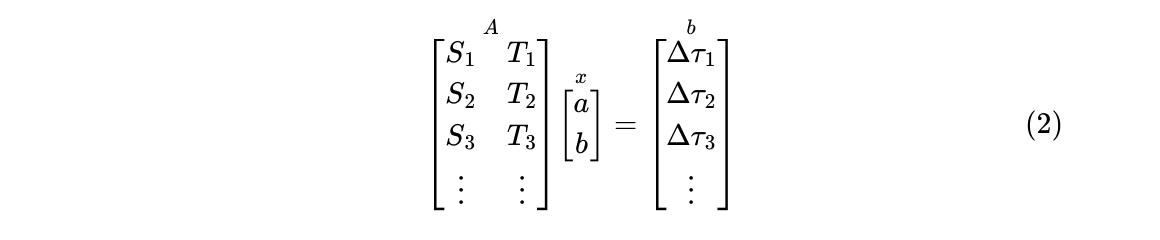
Step 8 is kind of magical. I knew about gradient descent, but I don’t have an easy way to calculate the derivatives necessary in this situation. While digging around for numerical methods of fitting data, I saw a mention of the downhill simplex method, which I’d never heard of. It does something similar to gradient descent but only requires the original function and not the partial derivatives. Even better, I found this lovely, single .h file C++ implementation of the algorithm.

The idea is that you give the algorithm a function and a set of starting parameters that can be passed to that function. It perturbs the parameters (in a very specific way), exploring the problem space, checking each result against the function until it finds the minimum value.

In this case, I just pick the intersection we found that was closest to the center of the image and then the intersection next closest to that one. (Pythagoras tells us we’ll always get an adjacent point and not a diagonal, no matter the rotation angle of the grid.)

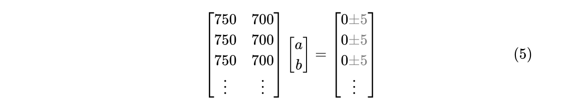
The parameters to the downhill simplex algorithm are simply the (x, y) coordinates of those two points. The line segment formed by those two points is actually enough to define an entire grid: the line segment’s length is the grid spacing and the line segment’s angle defines how the grid is laid out in the plane. So all that is left is to provide downhill simplex with a function that tests all of the other intersections we found, snapping them to the nearest point on some hypothetical grid, and reporting the error between them. Downhill simplex minimizes that error and finds the ideal grid that fits each intersection most closely. It returns two, sub-pixel (x, y) pairs that are ever so slightly different than the initial parameters, that now fit all ~650 intersections best instead of just those two.

The red grid overlaid on top of the original image in the final frame demonstrates several things:

• Downhill simplex is easy to use and gives good results.
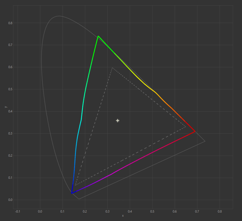
• The Schneider Componon-S 50mm f/2.8 lens has a remarkably flat field of view with essentially zero distortion, even at the corners.
• Even with all the junk in the line detection step, this algorithm is very resilient to missing or noisy data.

The earlier 1D version of the algorithm used the same steps 1 through 7 but had an extra three or four steps after to categorize things, find the scale’s axis, throw away intersections off the axis, order them, and check for consistent spacing between them. It was more brittle and couldn’t handle a single mis-detected point on the calibration slide (because of dirt, etc.).

So, one funny consequence was that the 2D algorithm continued to work in the 1D case and was more forgiving of bad data to boot. (None of those steps required the existence of a 2D grid; we only need evenly-spaced intersections.)

The size of each pixel can be read off directly: the length of the line segment is already given in pixels, and we know the length of the division in physical units a priori from the Amazon listing.

Here are some results for my particular IMX429 sensor and extension tube setup. These are the size of each pixel at the best focus position for each color channel:

• 2.8557 µm/pixel for red.
• 2.8552 µm/pixel for blue.
• 2.8503 µm/pixel for green.
• 2.8522 µm/pixel for white.
• 2.8798 µm/pixel for IR.

Something jumps out right away: red and blue have nearly identical pixel sizes! Keep that in mind for later.

Knowing that the sensor has 1936 pixels across, you can do the math and figure out that a picture of some object that is 6mm wide will end up ~3.4 pixels wider when taken with green light than it will with blue or red light. (For IR it’s almost 20 pixels narrower!) Assuming they’re aligned by the image center, by the time you get out to the edges, green will be off by almost two pixels. (For higher resolution sensors like the RPi HQ camera, this will be about 2x worse because it has about 2x as many pixels across.)

Instead of trying to correct for the effect by adjusting a bellows for each color channel, I think I’ll just resample each channel in software down by (up to) four pixels, realign them, and call it a day. That should clean up any color smearing at the edges and in the corners.

Focus Detection

The simplest metric for detecting an image’s relative focus is just taking the standard deviation of each pixel value in the image. That’s a one-liner in OpenCV, so it’s what I started with.

So we can see where our best focal planes are by walking the camera’s Z-axis forward one step, capturing an image using each color channel, and calculating the standard deviation of each image.

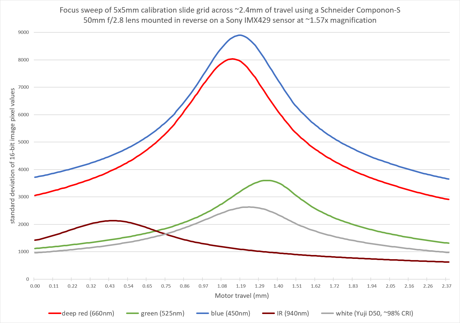
When you’re done, you get a beautiful graph like this:

Data is never that clean! Those are almost perfect Gaussians.

The amplitude of each curve doesn’t matter. That’s just the relative brightness of each LED (and QE of the sensor), with the camera set to manual exposure, so some colors were naturally dimmer than others.

The important part of each curve is the X position of the peak. That’s the ideal focus position. And the thing that jumps out immediately (and also agrees nicely with the pixel size observations) is that the Schneider Componon-S 50mm f/2.8 is achromat corrected.

I’ve never seen this mentioned in any datasheets or in any reviews. The red and blue would be even closer if my red LED was a “standard” red wavelength (620nm) instead deep red at 660nm. If you do the linear regression of each peak (except blue) and project a hypothetical 620nm LED onto the same line, it falls almost exactly on the blue peak.

So, 1/3 of my reason for using a motorized Z-axis has been solved by Schneider. (If only I could get my hands on an apo enlarging lens, I almost wouldn’t need the motor at all… but where would the fun be in that?)

Planarity

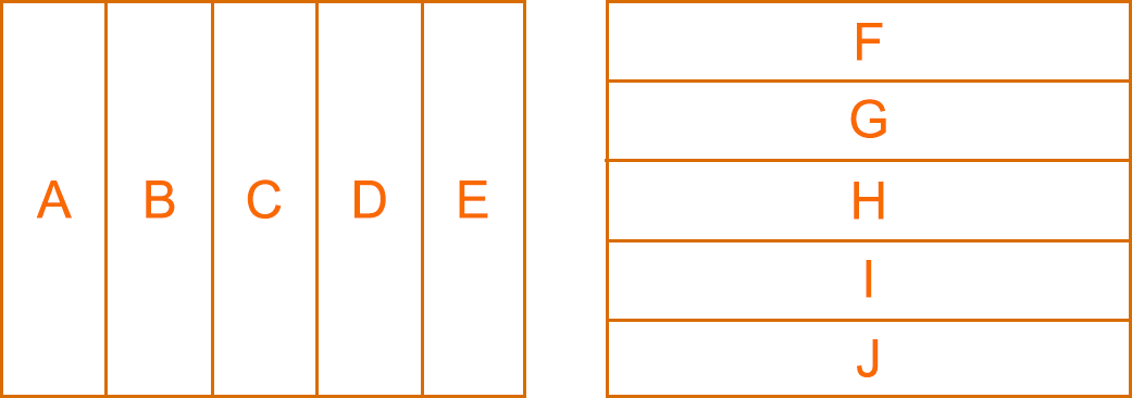
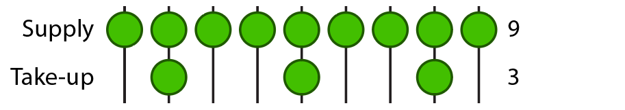
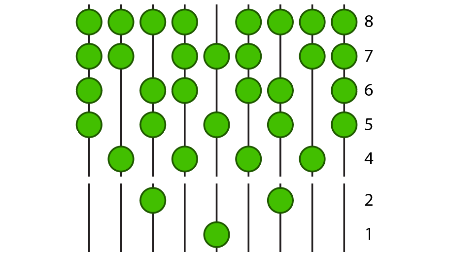
You can use the image’s standard deviation as a focus metric to perform one more cool trick. Instead of calculating it for the whole image, you can slice things into different focus zones:

Then, calculate the standard deviation for just those sub-images and plot them on the same axis.

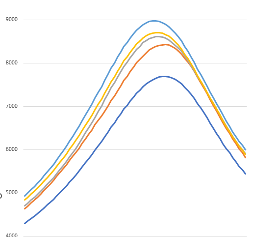
Here are zones A through E for a single color channel, taking an image at each Z-axis motor step:

If the subject plane was aligned perfectly with the sensor plane, all of those curves should have a peak at the same x coordinate, which would mean each part of the image would be entering and leaving focus at the same time. But it wasn’t!

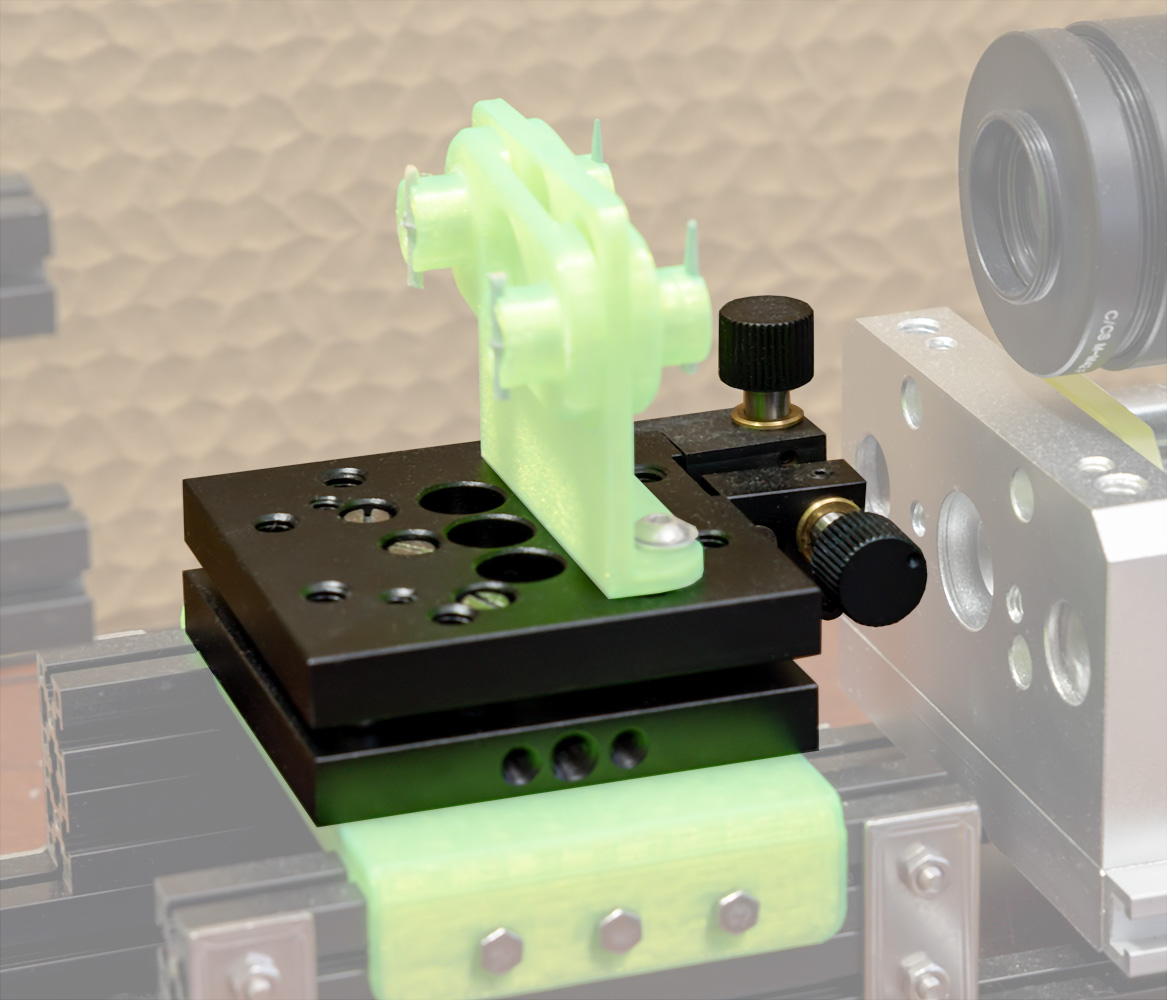
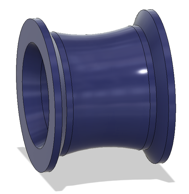
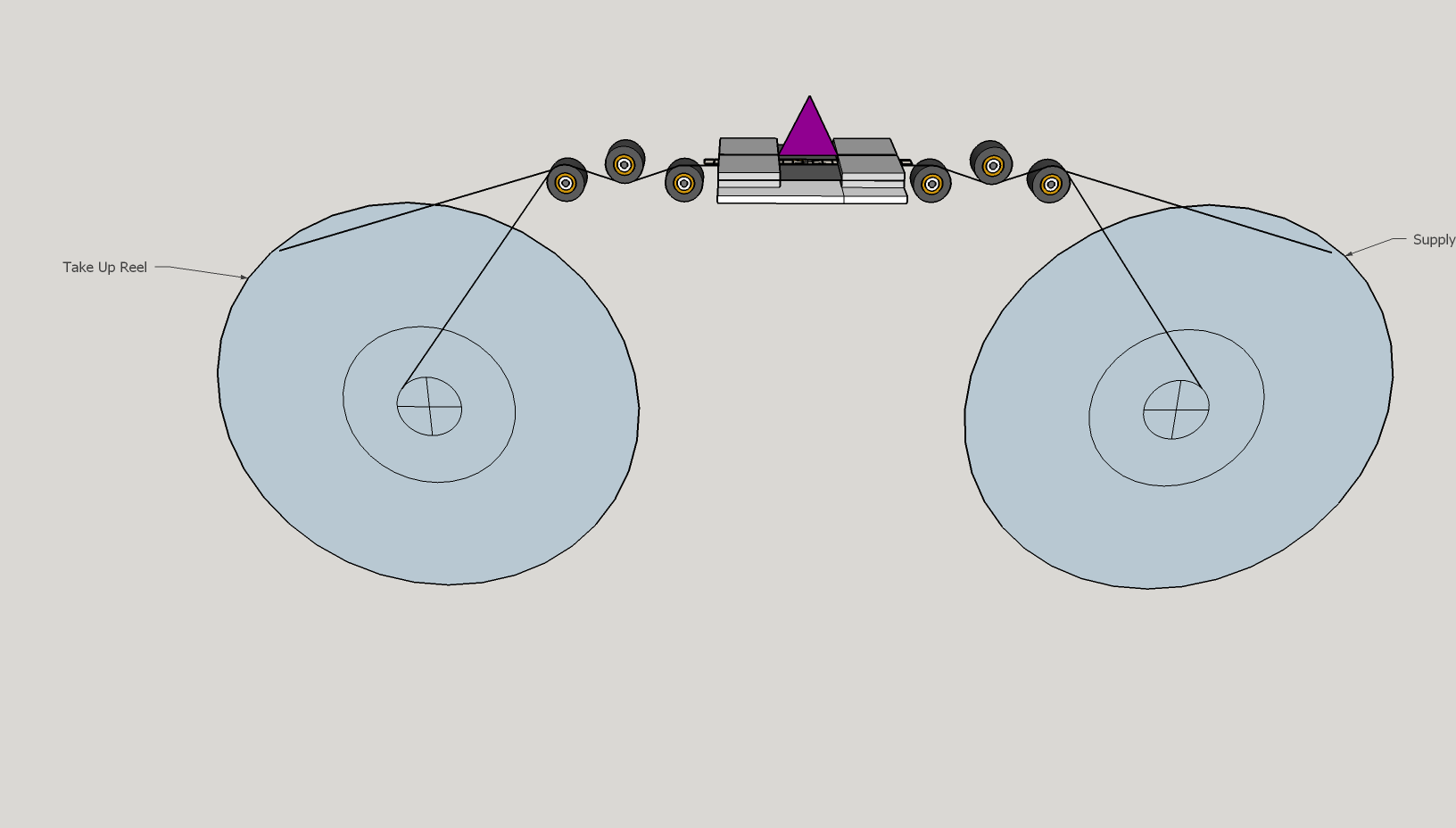
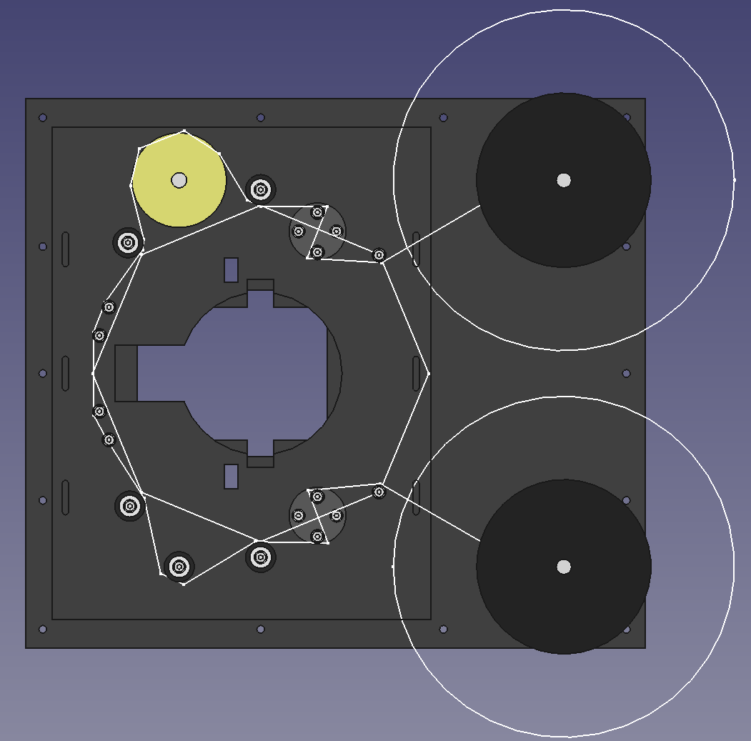
Eventually the film transport is going to be mounted to the same optical tilt/rotation table that I have the calibration slide mounted to now:

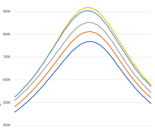
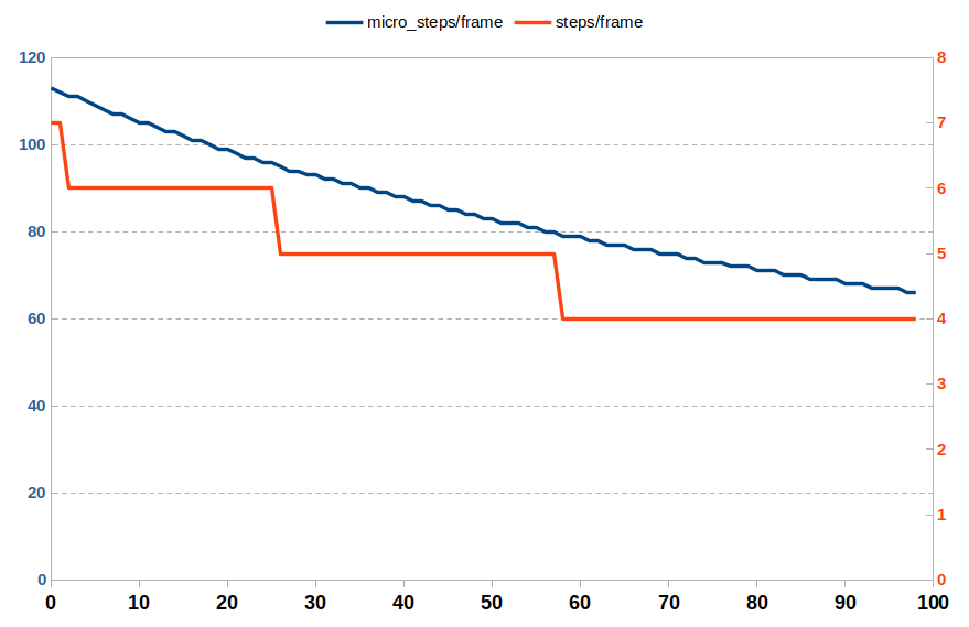
Those two knobs can adjust things by a couple degrees on a rotation and tilt plane, which is exactly what we need here. After a couple turns of those micrometer screws, I ran the planarity sweep again and got this back for zones A through E:

That’s a lot closer to being aligned with the camera sensor. I repeated the same for the other direction (zones F through J) and now images are sharper across the whole field of view than before (and the 2D grid pixel measuring algorithm started returning even more consistent results down in the nanometers).

There is an open question about how well the standard deviation metric is going to hold up with Kodachrome as the subject instead of a silvered calibration target, but hopefully I’ll be able to get things dialed in once I switch over to a proper film transport. Planarity seems like something you can dial in once and then forget about unless the machine gets bumped by something.

What’s Next

Focus detection isn’t quite “auto-focus”. Those graphs are still being generated manually in Excel. I want the focus sweep button to find the peaks and set up markers at the best focus positions so I can travel to each in a single button click. That is auto-focus and it’s going to require a little more algorithm design.

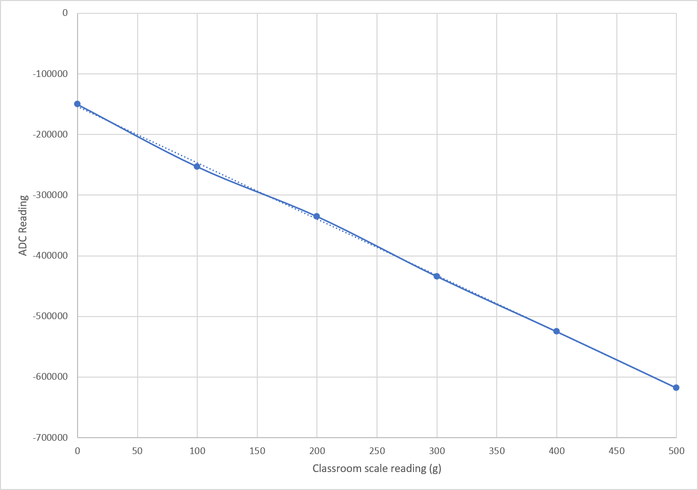
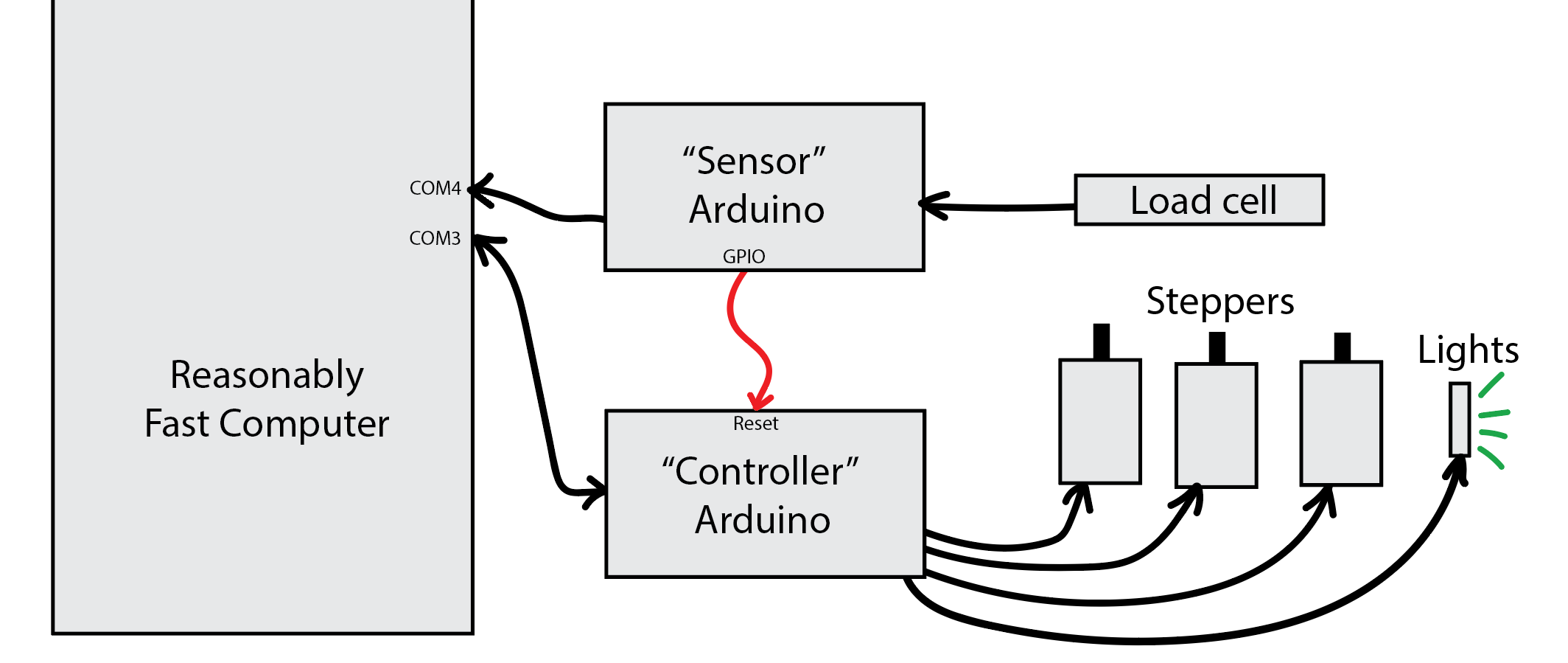
That’ll be in June and I’m planning to fill the rest with more integration work as I get closer to actually imaging film: I need to confirm that my software control of the motor (over my new communication protocol) is still as dependable as my early Arduino-only tests re: not missing any steps. I want to get the Arduino connected to the sensor’s GPIO so I can request exact exposure timing instead of just using the default video stream. And it’s probably time to see if I can’t read values from the load cell controller board that will eventually become part of the film transport.

[npiegdon]

@cpixip

The sensor will probably not feature 16bit resolution. It’s probably a 12bit sensor…

You were right. Despite my hopes for around 14-bits on the Pregius sensor, I’ve since found a spec sheet that shows LUCID’s Triton camera lineup only uses a 12-bit ADC to read from it. Oh well.

@PM490

Finally got around to make the port holes. Here is how it looks.

Those are some clean cuts. How did you do the off-angle cuts so nicely? When I was brainstorming how I might turn these cake pans into an integrating sphere, I couldn’t think of an easy way to hold them at those angles. As an alternative to off-axis ports, I took @cpixip’s advice that the sphere didn’t need to be perfect and instead optimized for the simplest construction steps: I put the entrance and exit pupils on a straight line and just inserted the smallest possible baffle between the two.

The little cone-like feature on the side facing the LED board is just to prevent the first light bounce from going directly back to the PCB. The other side is flat.

I overestimated the wall thickness of the pans a little. While milling the smaller exit port, it ended up with a razor-like edge and you can see a little wobble in the cutout where there just wasn’t any material left. I suppose the thin wall at the exit works out in my favor for getting it a millimeter or two closer to the subject.

The barium sulfate wasn’t as hard to work with as I was expecting. After some sanding, I sprayed everything with a white primer and then mixed a bunch of the powder into titanium white acrylic ink (mine was Liquitex brand). It still took 8 or 9 coats (and it probably wouldn’t hurt to do another five) before it was reasonably uniform looking.

And here it is fully assembled, on the rails, showing the front of the exit port. The mount (with the captive nuts) for the PCB is just held on with a couple drops of super glue for now. If that doesn’t last, I’ll use epoxy. Again, I was optimizing for speed-of-build this time.

This was kind of an extra credit mini-project for June. During some early testing with the Köhler stuff, I saw how much the direct lighting was accentuating scratches and other oddities in the film. If I’m going to save the wet-gate/chemistry portion of this project until the end, I wanted to have a good proxy in the meantime to help hide those defects while I was still working out the rest.

I probably shouldn’t have put my eye directly up to the exit port with (the dimmest of the) LEDs on, but I saw exactly what I was hoping to: a completely invisible baffle. The only discernible features inside the sphere are a faint seam between the two halves and the two little “tick marks” where the arms holding the baffle divide the seam line.

I can’t believe how homogenous this light is! I focused on my calibration grid, put the sphere as close behind it as I could, then removed the grid. The resulting flat, gray image had a difference of only 2.6% brightness between the center and the darker two corners. I think I might be able to do better by tweaking the alignment a little. The other two corners were only 1.8% darker.

The histogram is just a single spike with an (8-bit) std dev of 0.79. When you auto-contrast that out to the extremes, you can see the darker two corners.

I think I found a few dust particles in the lens. That’s the aperture blade pattern of the Componon-S lens. I’ve already tried cleaning the front without any effect. I hope they’re just on the back. But I expect they’re actually somewhere inside.

It’s mostly a non-issue because everything in that image is taking place inside two (8-bit) gray values.

[PM490]

@npiegdon

Those are some clean cuts. How did you do the off-angle cuts so nicely?

Start with a small hole,

and then use a step-bit, these worked great.

For the larger output port, did a jig to hold the cake mold and be able to rotate, while holding the dremel still with a milling cutter bit.

Then used the same setup with a sander bit to finished it clean.

Finished the edges with a light/fine filing.

[npiegdon]

Wow, so the side ports were done by hand with the step-bit?! I’m even more impressed. Nice work.

That jig was another good idea, too!

[npiegdon]

June/July: Early Direct Drive Transport with Load Cell

The ReelSlow8 has sprouted legs (and more). I wanted to get it off the table so I could run wires and have easier access when building the side arms.

My 7 year old started his summer break from school so my hobby time took another hit. I didn’t have enough to show in June alone, so I’ll do a June/July and July/August update instead.

Even then, instead of working on auto-focus I decided to finally tackle the pain point I experience anytime I need to carefully hold film in front of this thing for a test. It was time this film scanner could actually scan film.

I opted for the simplest film path I could imagine.

Direct stepper drive on both reels, two rollers as close as possible to the exit pupil of the integration sphere, and one extra roller for the load cell. The side-arms of the machine were designed with the MakerBeam very specifically to allow easy height adjustment for the steppers.

The rollers are (SLA) 3D printed to have two 693ZZ bearings pressed into the center. Then, you can run them right on an M3 bolt and use the nuts to fine-adjust the height. The curve in the center means they barely touch the edges of the film, as per usual.

The most interesting part is the load cell. If it isn’t the default choice around here for tension sensing, it should be and I’ll advocate for it any chance I get!

• It’s like $8 for a 1kg load cell.
• The SparkFun HX711 breakout board seems to include a few more components on the board to ensure good function vs. the boards packed in with the load cell itself (at least according to the reviews on both sites), so I tried that first.
• You can switch the SparkFun board from 10 Hz updates to 80 Hz just by cutting a jumper on the back of the PCB. (They advertise 80 Hz, but mine does about 92 Hz and I’m not complaining.)

There are complaints in the reviews that the data is especially noisy and you need to do all sorts of averaging over time, but those are use cases that need the accuracy all the way down to the least significant bits coming off the 24-bit ADC. For our purposes of roughly keeping film inside some, say 50g, tension window, we might need five of those bits.

When you plot the full-scale data with no averaging at all–just the raw data–look at how pretty this is:

ReelSlow8 Load Cell

Essentially zero-latency response and super clean data. The little bump each time the scale reverses direction is actually the static friction of the plastic piston against the cylinder breaking. You can feel it and, apparently, so can the load cell.

That little classroom scale is my plan for calibration. I haven’t gotten this far in the code yet, but having the app ask for a few measurements (maybe each 100g on the 500g scale to build a regression) before each scanning session should give sub-1g accuracy which is an order of magnitude more than I need.

[PM490]

Nice update, thank you for the information on the load cell, very interesting and something to consider.
I also like the roller design, very nice and simple.

@npiegdon

I opted for the simplest film path I could imagine.

I am only making this comment because on your design you have been very detailed; for a normal built, I would not even say anything…
One consideration on the current path S-path and air gate is that the film bow on the gate will change with tension, and that slight bow will change the focus point.
Additionally, on the pick-up reel side, as the reel fills up, the film angle to the air gate pick-up-side post will change through the reel, making the right side of the bow vary slightly, even when tension is held constant.

Understand in this case -with auto focus- that may not be an issue. And that the variations introduced by the pickup on the right side may be within the dept of field range, nevertheless, keep an eye for those.

My worst skill is building transport, and got lot’s of experience (what you get, when you don’t get what you want). To avoid the variation introduced by the filling pick-up reel, a simple fix is adding a roller post on the pickup side, mirroring-opposite to the one for the load cell, effectively changing from an S-path to a W-path.

Again, only making this comment given the extreme effort you have been doing on every little detail. Hope it helps.

[npiegdon]

@PM490

for a normal built, I would not even say anything…

I’ll take that as a compliment.

Also, these are great questions!

Regarding the film angle, this is a quick, not-to-scale mock-up of what I think you meant:

The darker blue shows that over the course of an entire reel, the angle will definitely change, introducing a cosine error term on the load cell roller (and one of the “gate” rollers). During calibration with the classroom scale, my plan was to try and hold it along the mid-line between the two extremes, so it’s calibrated on the average, halving the error.

Admittedly, talking about holding something by hand (and using a $3 instrument) probably demonstrates I’m not too worried about the results here. When I did a survey of all the recommended tension values I could find across as many different pro machines and archival reports, the tension values were all over the place. (Granted, these were mostly for 35mm film, but) I found–after converting all of them to the same units–all of the following mentioned as supported/recommended tensions: 200g, 300g, 170-450g, 170-850g, and “very little up to 340g”. So picking a conservative starting point like 200g seemed safe enough, but that I probably still didn’t have anything to worry about even if it ends up being off by, say 50%(!).

Also having the least experience with the transport (vs. all of the other relatively more known quantities), my plan was to cross that bridge when I came to it! My ace in the hole was that I intentionally used longer rails for the side-arms, so if the cosine error became a problem, I could just slide either the load cell or take-up reel back as far as another 8" or so. That would increase the length of the film path but also drop the cosine error fairly considerably.

Another design requirement I’m willing to bend on: out of the 39 reels I have to scan, 34 of them are 3" reels. If the couple 5" and 7" reels end up introducing too much error, I wouldn’t mind a pre-processing step of transferring them, piecemeal, to 3" reels for scanning. (Granted, I don’t want to do it, but I will if I have to, hehe. I already had that same workaround in the back of my mind in the event that the direct drive motors weren’t strong enough to turn the larger reels.)

As for film bow, this is probably my complete lack of experience showing. I had assumed that once you were wrapped around a roller far enough, the incoming angle wouldn’t matter anymore (given a particular tension level) and you could make assumptions about the behavior of the film from that point forward independent from anything that happened before it. And the “around a roller far enough” here could be modulated again by sliding things as far along the rails as necessary to reduce the cosine error. The “far enough” probably also depends on the diameter of the contact point on the roller. For very large rollers, I’d guess film bow is minimized/eliminated. For something like the LEGO cones in your design–which approach a diameter of zero–the tendency to bow out is probably accentuated.

Really, I’ve probably been puzzled over these questions longer than any other part of the project. Some pro scanners have dozens of rollers. Some have as few (or fewer!) than this design. Your own film path stood out as one that had an above average number of rollers and I’ve spent time scratching my head over what each one might be for.

I’d dragged my feet on this part for as long as I could (something like five years ) and it was finally time to commit something to paper–good or bad–just to get a move on. I was hoping the first iteration would get close enough, but I’m not so confident that I’d be surprised if I had to tear most of it down and try again.

The eventual addition of a full-immersion wet gate only adds the requirement that the film near the light source be convex (w.r.t. the camera), which the current S-shaped path permits (even if you’d probably have to slide those two elements farther down the rails toward the camera to make it more feasible). But your W-path suggestion also meets that requirement, so adding that extra roller in the event that film bow becomes a problem would be a good workaround.

All of that is a long-winded answer to say I am much less confident about this part of the design and am mostly crossing my fingers, hoping for the best, and am planning to tackle problems as I run into them.

[PM490]

@npiegdon

I’ll take that as a compliment.

Yes, it is

Here is my totally empirical summary, the point of view below is framed by these.

• Angle of bend around a post or roller adds tension to the force needed to move the film. In my case, I had the rubber rollers with bearings (little friction) and the loose-lego-conical-posts without bearings (more friction). In general, the larger the bend, the more friction.
• Old film is less flexible. Larger tension was needed to flatten the film on the air-gate-posts. Less tension would bow the film. Thought this could even be used for narrow focusing. In my case, the space between the gate-posts is larger, because I wish to capture almost 3 frames of 16 mm (one frame with more than two halves), consequentially the play bowing was more noticeable.
• Because of the old film lack of flexibility, and the narrow lego-posts it was necessary to avoid large angles about a post, or risk the film breaking at the perforation (experienced it) when using more tension.
• Eliminating the variability of the increasing/decreasing spool takes away one more uncertainty. The less uncertainties with areas I have the less know-how, the better.
• The transport is intended to be 16 and 8, without any changes other than software. This is an aspiration, but the preliminary results were promising.

With that thinking framework, a few comments.

@npiegdon

The darker blue shows that over the course of an entire reel, the angle will definitely change, introducing a cosine error term on the load cell roller (and one of the “gate” rollers). During calibration with the classroom scale, my plan was to try and hold it along the mid-line between the two extremes, so it’s calibrated on the average, halving the error.

I was less concerned about the load-cell effect of the supply-reel angle changes, mostly because my lack of know-how on the cell, but you have a point.

@npiegdon

As for film bow, this is probably my complete lack of experience showing. I had assumed that once you were wrapped around a roller far enough, the incoming angle wouldn’t matter anymore (given a particular tension level) and you could make assumptions about the behavior of the film from that point forward independent from anything that happened before it. And the “around a roller far enough” here could be modulated again by sliding things as far along the rails as necessary to reduce the cosine error. The “far enough” probably also depends on the diameter of the contact point on the roller. For very large rollers, I’d guess film bow is minimized/eliminated. For something like the LEGO cones in your design–which approach a diameter of zero–the tendency to bow out is probably accentuated.

I used two kinds of post, the narrow lego (conical only touching edges) and the wider rubber-roller-bearing (flat full contact). With old film, I saw bowing on both. The rubber is probably closer to your design, but on yours, these are only touching the edges, I think the opportunity to bow is there… similar to the lego (only touching the edges also). All speculation, testing is king.

Based on past experience (which may not be relevant to your rollers) I would expect some uneven bowing (very exaggerated in the illustration).

The angle on the left side does not change, the angle on the right side changes, providing an opportunity to bow differently than the left side. This may be so minimal that it may not matter, again, just mentioning it given the attention to detail on your work. Just keep an eye for it, and see if it matters.

@npiegdon

Really, I’ve probably been puzzled over these questions longer than any other part of the project. Some pro scanners have dozens of rollers. Some have as few (or fewer!) than this design. Your own film path stood out as one that had an above average number of rollers and I’ve spent time scratching my head over what each one might be for.

Same here, with the added camera sensor and sensor software learning curve.

A big difference in the path is the type of motor used, probably cannot oversimplify/equate film paths of different motor kinds.

I’ll shed some light on my path design, a path for steppers. In very old posts, I started with an inverted V, with 3 rollers on each side of the gate.

Then came the proof of concept for the transport with Tof.

@PM490

Here is how the SnailScanner V0.1 looks.

First reference to load cells was at the post of the Tof (square path above) from @friolator, but I did not rethink the initial inverted V path.

@friolator

The low budget way to do the tension sensing would be a dancer arm and a potentiometer. But if you’re looking for something cool, I think you should check out load cells.

The first path, inverted V, is nice and symmetrical, and the 3 rollers take away any variations of the spool-size-changes, and two load-cells in the second roller of each side would give perfect feedback to control the steppers. For precision, one of the gate-edge-rollers can be numerically encoded. As I write, I think this is a neat transport alternative, and one that I may revisit down the road.

The one turn-off was that it was large, in order to make space for the large sphere, plus two large reels virtually in line. That’s when I started playing with ideas of a wrap-around path, to keep the project at a reasonable size for storage.

Then came the ToF path, which is virtually a square, and provided experience on turning old film.

The new path is based on an octagon, and it is virtually symmetrical between the supply-side and pick-up side. The pickup side has the capstan, and supply side has a roller where the capstan would be, which is the only difference (the middle roller in the 3 at the bottom.

Tried to eliminate variations induced by spool-size, both sides start with an entry post (right side of the octagon). Both sides have identical dancing-potentiometer, the entry-exit angle of the potentiometer is fixed by the entry-post and the first roller (from right to left). The next side of the octagon is the capstan (on the top) and the dummy-mirror-capstan, the three rollers at the bottom. The two left sides of the octagon are the gate.

The large sphere needed for 16 mm target (more than one frame) takes a lot of space. When working on the failed prototype, one of the takeaways of the experience was the fragility and rigidity of old film (have a couple of the 16mm close to 70 years old). So was looking for a compact arrangement with a path minimizing sharp bends. The entry post, with large spools are the only ones would be over 90 degrees (the old 16 mm film is in smaller spools, and the angle would be far less than 90).

So in short, all those rollers help make the transport plate a bit smaller, and lesser the film bending.
Please, don’t follow me, I’m a bit lost… but making good progress (paraphrasing Yogi Berra).

I suggest you change nothing until you test it, and use the information provided as things-to-keep-an-eye-for. Perfection is enemy of the good.

[npiegdon]

@PM490

Here is my totally empirical summary, the point of view below is framed by these…

This kind of freely shared experience is the reason this forum is great and how it has become a veritable dragon’s hoard of collected wisdom for these kinds of project.

Film bow wasn’t on my radar before, but it is now. I’ll keep an eye out for any problems while I’m testing things. Thanks again for sharing!

[friolator]

@PM490

20230714 Octagon Transport1051×1037 19.4 KB

This is not unlike the Imagica 3000V transport. It was a scanner from the late 1990s - very slow - designed for digital intermediates. If you think your scanner will run slow, remember that the 3000V took 30 seconds PER FRAME to scan 35mm at 4k! I had one of these as the basis of my first conversion project, but ultimately moved to a different platform. but the basic transport is not unlike your new layout:

[npiegdon]

July/August: Direct Drive Transport (part 1)

Last time, the wires for the transport steppers weren’t even connected. Now, the ReelSlow8 can reliably maintain tension while moving.

The picture hasn’t changed much; just fewer loose wires, the classroom scale is still there from calibration, and the E-stop finally found a home where it’s easier to press.

That said, there are some really cool details where things have started to come together in a way that feels like more than the sum of their parts.

Load Cell Linearity

I wanted to get an idea about what sort of curve I was going to need to model in the software to convert raw ADC counts from the load cell into a tension measurement. So, I mounted the classroom scale close to the same position and angle the incoming film would normally be coming from. Connecting the other end of the little snippet of film to the take-up hub, I can pull the scale out to some number and lock it in place with a screw.

Testing at each 100g on the scale, averaging a few hundred readings at each point, these were the results:

That the linear trend-line is almost hidden by the data itself across the entire range is about as good as you could hope for. So, now that I know the slope for this particular load cell, all the app needs to do is “tare” using a single 0g data point. Nice and easy.

Key takeaway: treating the load cell data as perfectly linear seems like a safe assumption.

Load Cell Creep

Something you notice when watching the ADC counts rolling in at ~90Hz is that those lower 10 or so bits (of 24) are always walking around all over the place. It’s not just white noise, it’s sort of shimmying around over time. I’d also noticed that just after making a large tension adjustment with the classroom scale (say, more than 100g from where it was before) that over the next couple minutes, the random walking behavior in the data seemed to trend more in one direction than the other.

To try and characterize this creeping behavior, I performed the following experiment:

1. Remove everything from the film path (0g tension) for >24h.
2. Use the classroom scale to tension the load cell to 200g.
3. Leave it at 200g for >24h.
4. Remove everything (0g again).

Then, immediately before/after and 5min before/after each of those steps, I would take an ADC reading.

I was happy to find that the wiggly lower bits were less trouble than they appeared to be. I never saw any deviations larger than 1.7% (of the 200g), so maybe a 3.3g deviation in the worst case (reading immediately after a large change when the load cell has been in a different position for a long period). In most situations, the error was below 0.8%.

My own target when moving the film is to maintain a range of about 15g from my desired set point, so the worst case is already inside my noise allowance. To improve things, I could pre-tension the machine to my typical running set-point the night before I plan to use it.

Key takeaway: don’t plan on splitting grams, but our application never needed to in the first place.

Film Path Safety

So, these reels are precious family relics. I want it to be near-impossible for my buggy code to do any harm to this stuff. Beyond the E-stop button (which physically severs all motor current), I wanted something automatic in-place that could react faster than I can.

I wasn’t quite sure how to get the kind of guarantees I was looking for from a single Arduino. I’ve been avoiding interrupt-driven microcontroller code just for ease of reasoning, so reading from the load cell involves polling and busy waiting. For similar reasons, I’ve opted to “bit bang” the actual step pulses to the stepper controller boards rather than using something like PWM and crossing my fingers that I get the timing/counting right.

So a natural architecture fell out of my (made-up) requirements that ended up working well for the safety I was looking for:

The “controller” Arduino sits and waits for messages, responding to each one in turn. The “sensor” microcontroller just has the fire hose of load cell readings dumping into its serial output. By adding a single command to the sensor board, I was able to get exactly what I wanted.

One of the first operations you perform when launching the desktop app is to tare the load cell by averaging a hundred or so readings when nothing is touching it. Once the app knows the appropriate zero-point (and constant intercept), it sends the sensor board a min/max limit. From that point on, if it ever sees a reading above or below that range, it immediately pulls the reset pin on the other board. The initialization routine on the controller board sets the motors to 0% current, so the tension is dropped to zero.

My favorite part of this scheme is the low-latency. No USB round-trips, no queued serial messages, and no I/O delays inside the OS. Microseconds after the load cell knows about the problem, it’s stopped.

I’ve already accidentally tripped that safety mechanism a half-dozen times and it’s worked flawlessly every time. It’ll trip just from tugging on the film with your finger.

The controller board also sends a startup message when it is reset, so the desktop app can interrupt its current operation (if any) and show a big, red warning message that requires user intervention before continuing.

Since I got that up and running, my worries about accidentally destroying these family memories have been allayed.

Key takeaway: it’s better to put the time in on this kind of stuff up front before an accident happens, if only for peace of mind.

Simple(r?) Super-8 Sprocket Detection

I’d been planning to use a scheme like @cpixip’s Simple Super-8 Sprocket Registration as most of the criteria there (sub-pixel registration done in a separate pass, etc.) applies to this machine as well.

My app doesn’t stop on frame boundaries yet, but I had a shower thought the other day about a method that requires many fewer calculations and steps to get a rough sprocket hole position and decided to try it.

It relies on the assumption that the film will be properly exposed so that sprocket holes are the only “burned out” areas in the image.

The shortest explanation: calculate the center-of-mass of only the over-exposed pixels. That’s it. That’s the y-coordinate of your sprocket hole’s center.

Here, red pixels are over-exposed. And the blue line is their center of mass.

If you haven’t seen the calculation before, there’s not much to it:

var moment = 0
var total = 0
for each line y in the image
   var count = number of over-exposed pixels in that line
   moment += count * y
   total += count

var centerY = moment / total

I already needed to walk the entire image for a different process anyway, so I test all the pixels. But, to save effort or if you are zoomed out far enough to see beyond the edges of the film, you could employ the same vertical band technique from cpixip’s post.

And if you’ll be moving close to a frame at a time before checking to see where you ended up, you’ll only ever have one hole visible at a time so, again, you’re already done. Otherwise, you can count the number of lines since the last time you saw any overexposed pixels and after some threshold (20 lines? 40?), start accumulating a new center-of-mass. That will find all of the sprocket holes.

The only weakness is that it gets a little inaccurate when a hole is only partially visible at the top/bottom edge of the sensor frame, but that’s exactly when you need the precision the least.

---

More Soon: There is a lot of exciting math involved in direct-driving two steppers to maintain tension (without a capstan and while still getting useful movement done), but it’ll take a couple days to put together the visual aids and record a video. So, I’ll split off this grab-bag of unrelated progress so I can focus on just that part next time.

[PM490]

Great update, thanks for sharing.

@npiegdon

There is a lot of exciting math involved in direct-driving two steppers to maintain tension (without a capstan and while still getting useful movement done), but it’ll take a couple days to put together the visual aids and record a video.

From my experience (experience is what you get, when you don’t get what you want) with Time-of-Flight sensors, I did try a pure math approach to moving without capstan, and it worked fairly well, except one my my goals of the project was to scan film without sprockets (develocorder), then loosing a position reference to work with.
Using 100:1 geared steppers (99+104/2057 to be exact), and measuring with a caliper each spool, and the film thickness, the PICO was able to hold a fairly steady movement for a few dozens of frames without any feedback loop.
You have a better transport setup, tension feedback… but the math says that with large diameters spools, will be challenging to hold precision with the 200 steps/turn of a normal stepper, even if using 1/16th micro-steps (what I had available).
A 50 mm diameter reel translate to about 5 stepper-steps, or 80 micro-steps, per Super-8 frame. Granted, error can be corrected digitally panning from the sprocket reference (when sprockets are available).
After trying, I have a healthy respect for the tolerances involved in the movement of 8mm film, actually seeing some even with a capstan. Godspeed mate.

[npiegdon]

Thanks for the encouragement; I agree with all of that!

I couldn’t imagine attempting it without feedback. (I’m still impressed by your ToF results!) Larger reels would definitely make it more challenging to stay inside my error margins. And 1/16th steps are the largest I’ve ventured for doing anything close to precise. 1/32nd seems to be a sweet spot for coarser moves with the smaller 3" reels.

The 10% or so over-scan shown in that frame above gives enough leeway that only having a mostly-centered sprocket hole should be good enough. That’s one of the reasons I’m not too worried about the precision of the center-of-mass tracking algorithm.

It’s been funny: you and I have been doing some of the same detective work in parallel. While you’ve been posting about the non-linearities in the new SnailScan transport, I’ve been marveling at how similar the sorts of oscillations I’ve been seeing on this side have been, too. Even just these old plastic reels seem to have a bit of lopsidedness to them, not to mention all the parts that I’ve made.

The neat, feedback-based, adaptive-style math I’ve got working is just for the tension half of the problem and not for getting frames centered yet. But the way I was able to break down the problem, I did most of the hard part up front, so centering on the frames should be the easier of the two. (Famous last words!) In the meantime, I’m still pretty excited at how well the first half worked out. It ended up being a very simple scheme (after trying to over-complicate it for a week or two) that I hope to explain in detail shortly.

[npiegdon]

July/August: Direct Drive Transport (part 2)

It took a few weeks of trial and error to come up with the following, but it was a lot of fun. You can see half a dozen blind-alleys, over-complications, and wrong answers in my notes before it all shook out into the simple form in the rest of this post.

Interleaved Steps

Like I mentioned last time, I’ve been trying to write my Arduino code with an emphasis on being able to read it straight through so I won’t have to do so much tricky reasoning about what state things are in or which interrupt should be firing next, etc. So, when it came time to step two motors simultaneously at different rates, rather than attempt to do it with PWM units in hardware (where I’m less confident about stopping them exactly at the right step count), I wondered if there might not be an easy way to do it manually.

I’ve got all the stepper motor’s “step” pins connected to the same AVR “port”, so they can be updated simultaneously just by setting a single 8-bit value in the code. Which motor(s) get stepped depends on which bits are set when you change the value. You end up with something like this:

PORTF = mask;
delayMicroseconds(d);
PORTF = 0;
delayMicroseconds(d);

Whichever motors are selected in your bitmask will get stepped, the rest will sit still. You can do this in a loop or with some other timing mechanism to handle acceleration and deceleration, but it always comes back to the decision of which motors to step and when.

So, starting with an example where we’ve determined we need to advance the supply reel 9 steps but we only need to advance the take-up reel 3 steps (say, to decrease our film tension a bit while nudging the center of the frame a little), you could imagine we could choose our bitmask for each successive step like this:

The motor with the larger number always gets stepped every cycle. And, ideally, you find the right spacing for the motor that needs to move fewer steps so that the move is as smooth as possible.

At first, I was worried that writing the code to do that would be full of special cases, keeping track of different sub-patterns, worrying about round-off, and all sorts of other details. I mean, when you look at the rest of the ways to fit every combination of fewer pulses into the same 9 steps, it seems like the code to generate all these (nice, symmetrical) patterns would be tricky:

And that’s to say nothing of the real world cases where you might be moving hundreds of steps at a time. (Every fifteenth pair, there is a group of three steps on the 242 line in this example):

While doodling these step patterns in my notes, I eventually noticed some similarities to modular arithmetic. Adding another multiple of the smaller number each cycle, dividing it by the larger, and producing a step anytime the rounded result increased by one started to produce these lovely shapes without any regard to keeping track of… anything else.

It was an easy answer that worked with floating point math and round-off, but the Arduino is an 8-bit processor that doesn’t like doing floating point math if it can help it (and you always have to worry about numerical stability with those sorts of solutions). So, I played with the idea a little more until I found an all-small-integer solution that ended up even simpler.

Here it is, for posterity:

unsigned short s = floor(larger / 2)
for 1..larger
   s += smaller
   if s >= larger
      step both motors
      s -= larger
   else
      step larger motor

That’s it. One addition, one comparison, and maybe one subtraction per cycle. For any sensible number of steps, all the math fits into 16-bit numbers, which avoids generating an onerous number of AVR instructions. And there are never any large numbers that might overflow.

So now we can make arbitrary simultaneous interleaved moves. Now the question is how many steps should we be moving?

Maintaining Tension While Moving

Advancing the supply reel reduces tension. Advancing the take-up reel increases tension. After moving S supply steps and T take-up steps we get some change in tension, Δ𝜏.

To relate these, let’s introduce constants a and b with units of “change in tension per step”, which lets us write:

Really, a and b vary slowly over the course of the entire reel, but are relatively constant across many successive frames. While advancing, a is negative and b is positive. (Again, supplying film reduces the tension and taking it up increases it.)

If we can find good (current) values for a and b, we should be able to move reliably while maintaining (or deliberately changing) the tension on the film. One solution might be to stop scanning every once in a while to do a recalibration: make a small move or two on both reels, one after the other, measure the tension change between moves, finding a and b directly. But, short moves are more susceptible to all the sources of noise.

The good news is that there is an easy way to get much better accuracy without even interrupting the film scanning.

Every time we move, we get another set { S,T, Δ𝜏 } which, ideally, we could use to help narrow down a and b. Because this is a noisy dataset, there will never be an exact solution. Instead, we estimate them by finding a least squares fit across all our recent measurements.

(Geometrically, this boils down to finding the best-fitting plane in three dimensions, with one point per recorded motor move. Each point’s distance from the plane is an “error” term. The error is squared to–among other things–always make it positive. Then, the algorithm finds the best plane that minimizes the combined squared error of all the points.)

Least squares fitting is a built-in operation in OpenCV, so long as we can get our problem into the usual Ax=b form:

The only mildly interesting part here from a code standpoint is interleaving the S’s and T’s in an OpenCV Mat with two columns. Once you’ve got everything stored in the correct size cv::Mat, you just call:

cv::solve(A, b, x, cv::DECOMP_SVD);

Then, read the a and b coefficients straight out of the x Mat.

Despite a lot of noise in the measurements from all the non-linearities and imperfections in the ReelSlow8’s construction, the best fit against the previous dozen or so moves produces remarkably stable estimates for a and b.

With those in hand, we can now make the next move. We start with however many desired supply reel steps S (say, our guess for what it’ll take to reach the next frame), the current tension 𝜏0, and the desired tension after the move completes 𝜏1. Using the latter two, we can find the desired change in tension:

In the ideal case (where a move always lands exactly at the same tension as before), this would always be zero. But, in the presence of system noise and integer stepping, there are usually a few grams of under- or over-shoot that we also need to correct for.

Now we can solve equation (1) for T and find the number of take-up reel steps required to move how far we want while maintaining the tension we want:

In practice this works well over distances up to whole frames with the tension barely fluctuating over the course of the move!

That said, there is a danger: the estimates are so stable and the results so consistent, that it’s important not to make the same move over and over (say, moving exactly the length of one frame).

An example is illustrative: if it takes 750 supply reel steps and 700 take-up reel steps (in this particular area of the reel) to advance one frame without the tension changing (besides the usual noise sources), once your history buffer wraps around, you end up trying to solve:

Even though you have many equations and only two unknowns, the redundancy between them leads to a degenerate (or singular) matrix. All of those points that are being fit to a plane fall on the same line, which means many different planes could intersect the line equally well.

In this case, the coefficients could be -5.5 and 5.9. Or they could be -11.0 and 11.8. Or any other multiple. There is no way to tell! The coefficient estimates can become suddenly unstable once the initial “bad” points have rolled off the end of the list of historical points.

The solution is easy: just vary something. Instead of moving directly to the next frame, get there in two moves and vary the desired tension between them. If your working tension for image capture is 190g, have the intermediate move target somewhere around 140g, just to get a little “contrast” in the readings. Just about anything different will keep that best-fit plane from spinning around the degenerate line.

Once you take that caveat into account, the estimates provided by this model land the moves (at 1/32nd micro-stepping, directly driving 3" reels) within a few grams of the target tension after any number of steps you like, every time.

The best part is that it’s completely adaptive: over the course of the reel, the coefficients will slowly shift as the amount of film changes on each. The only real question is how large should the history buffer be? Too short (3 or 4 samples?) and things will be more susceptible to noise. Too long (60 samples?) and it might adapt slower than the coefficients are actually changing. A dozen or two movement history data points has worked well.

One last detail: there is a bit of a chicken-and-the-egg problem with the coefficients. How do you start gathering move data without knowing how far it’s safe to move? The easiest answer is to just use the weaker direct measuring scheme mentioned above, once, at the start. While longer moves provide more steps to average the tension changes across, it only takes a couple very small moves to get a reasonable basis to start the least-squares operation from. I have my app do an { S=5, T=0 } move followed by an { S=0, T=5 } move (disregarding any desired tension, just recording what happened after each). Because those are orthogonal as far as the solutions to the linear equation are concerned, it has worked as a good starting point. From there I use the estimates to walk a dozen supply reel steps, then fifty, and by that point the least-squares solution has locked on pretty closely and you can move however you like without fear.

ReelSlow8 Tension Demo

What’s Next

With good sprocket hole estimates and the ability to move smoothly while maintaining tension, the last step before this machine could be said to actually do something useful is figuring out the number of steps to center the next frame in the camera viewport.

My guess is that an adaptive, best-fit scheme will work for that, too! We’ll find out soon.

[PM490]

Thanks for sharing the insight of your project, it is great to see other projects perspective.
Math is not my strong area, so I may not even be getting 100% of your post. Most of what was not used frequently is hard to access

I also had to deal with the interleaved steppers, first for the two-stepper transport. At the time, as I shared, the ToF was to provide the reel radious, from which it would calculate the corresponding perimeter of the circle and steps needed for a frame size over that perimeter.

When ToF did not work, I tested how it would work with math & measurements (no feedback).

The (correction) diameter changes are somewhat discreet, and for the supply reel in the form of:
Diameter of Empty reel + Film Thickness * 2 * Number of Turns

Easy to keep track of what turn one is in, or calculate. There are less than 100 turns for the typical 50 ft Super 8 reel, so it can even be implemented as a constant array.

There are some complications with the fractions of frames/steps, but is workable with code and variables.

The TakeUp side is the inverse horizontal flip of the Supply side.

[PM490]

One key difference I should have mentioned for context is that the load-cell does not have the elasticity (implied safety margin) that the dancing potentiometer does (spring or bands).

On the interleave approach, of the 3 steppers (capstan, pickup and takeup), the key is to find the one with the smallest radio (at any given time), and set the pace for the steps based on that scenario. At first, when using the 50mm encoder capstan, the takeup and supply had the scenario of the smaller radio (pickup at the start, and supply at the end).

The loop was set to provide those with the opportunity to have the ratio of steps at the smallest radio. In the large capstan scenario, two possible steps of takeup or supply for one of capstan. Then at every capstan step, the pickup and takeup tension is checked to decide if the corresponding stepper needs to skip the step. It is not elegant, but works extremely well, and tension is virtually constant (keep in mind all steppers are geared, and the changes are very small).

In your case (smaller number of steps than the geared, and no tension elasticity) I am unsure if the above approach would work. Given the quick reaction time of the load cell, I think it would with microsteps, but certainly your approach is more elegant.

Great work, and thanks for sharing the insights, certainly great reading.

[npiegdon]

September: First Footage!

Advancing to the next frame was like the tension math but only one variable instead of two, so it boiled down to keeping a simple running average of the last dozen or so estimates and errors. And… that was the last task before hitting minimum viability.

Right now it only uses a single focus point instead of per-channel focus, uses an integration sphere instead of Kohler lighting + wet gate, the software is still rather underdeveloped, and after these three hundred or so frames, a couple nuts loosened themselves to the point of having to stop the capture early, but now it does something!

This is very early and I haven’t pinned down even half of the processing chain yet, but here is some footage of my grandfather showing off a silly birthday gift back in 1976. The comparison on the left is from the 480i MiniDV camcorder-pointing-in-a-mirror-box transfer that a couple of my uncles did back in 2011.

Notably, this footage was quite faded and I’m excited to see how much of that information was still hiding in there:

8mm 1976 Birthday Party, Comparison

Again, this isn’t anywhere near final, but that is motion stabilized, color corrected, temporally denoised, and finally motion interpolated.

Temporal Denoising

The real star of the show here is NeatVideo’s temporal denoising (set to use the maximum of all five frames before/after):

That is pulling out details you never would have known were there! It wasn’t even clear that wall had wallpaper and after denoising, the pattern is perfectly legible. The double-quote on the t-shirt went from a fuzzy square to clearly double tick marks. The curtains went from “I think there is a pattern…” to being able to pick out details in it. So cool!

Color Profile

The color correction is 95% just done by eye right now. But, now that I’ve established good exposure times for each channel, I was finally able to dredge out my old Wolf Faust K3 Ektachrome calibration target and try to capture an ICC profile.

The machine is set up for scanning 8mm but it’s a 35mm calibration slide… so it took thirty four(!) separate captures, meticulously moving the helping hand that the slide was clipped into a little each time. Worse, I couldn’t find anything that didn’t fail to auto-align the images, so I ended up doing that by hand, too.

CoCa (alternate link) v1.9.7.4 (using Argyll v2.3.1) is free and can read IT 8.7 targets (and the spectral data file that was included with the target) and generate a profile that can turn raw camera pixels (left) into something calibrated (here, sRGB on the right):

Really, it’s a testament to the Pregius sensor that this isn’t doing a whole lot more than applying the 2.2 gamma ramp I requested at the time of profile creation. The response curves and gamut chart (generated by the also-free DisplayCAL) don’t include any surprises:

(The inset triangle is sRGB.)

Outside of the tiny wobbles (which I don’t know how to distinguish from measurement error), it’s almost a “perfect” sensor response.

In addition to generating those charts, DisplayCAL can also convert the ICC profile into a .cube LUT file for use with video editing software.

Because the response is so close to just adjusting the gamma by itself, I could probably leave this step of the color correction process out, but I am encouraged that anything my “deep red” LED might be bringing in strangely/non-linearly is getting corrected before the rest of the manual color correction process.

(As it turns out, once I took the time to catalogue my family’s footage into a spreadsheet of all my upcoming work, there was a lot more Ektachrome in there–about 30% of the collection–than I realized. So, even if this profile is only useful for that type of film stock, it was hopefully time well spent.)

Next Up

I’ve taken a slight detour to do better pre-registration before the motion stabilization step. At 0:10 in the video you can see some shaking. That was a place where the motion tracking (Deshaker 3.1 at the moment) couldn’t cope with the raw frames jumping all over the place so it fell back onto how they were captured. Right now if you watch the sprocket holes from the raw capture, the frame-to-frame movement can be upwards of 60px, jittering all over the place. (That’s about what I expected from my frame advance code. There is plenty of over-scan to compensate for the inaccuracy.)

So now I’m thinking I should at least try to make it easier on the stabilization software by getting the sprocket holes within a whole pixel of the same point by simply translating (and cropping most of the over-scan) before writing the TIFF to disk. Translating on whole-pixel boundaries (with no rotation or scale) is lossless, so it should be safe. On top of reducing the demand on the stabilization algorithm, it’ll hopefully save a little disk space, too, without the redundant bits of previous/next frame above and below.

So that will be some more fun computer vision algorithm work to beef up my center-of-mass based sprocket detection into sub-pixel accurate sprocket hole edge-finding. (So far it looks like it’s just going to be a few more applications of robust least-squares again. RANSAC is a powerful tool and a one-liner in OpenCV!)

While I’m tracking down sprocket holes, I also want to build a software tool to help me align/calibrate the angle of the film in the holder. Once those nuts started to loosen, the frames started to tilt more and more, so having a little gauge in the UI to watch for that failure condition will be helpful. The two rebuilt roller assemblies right in front of the light source use springs and Nyloc nuts now and can be adjusted easily with a single turn of a screwdriver instead of trying to hold/tighten two nuts (above and below the bearings) simultaneously. It’s a huge quality of life improvement.

Beyond that, I’ve got some fit-and-finish work to do on the machine and the software before it’ll be ready to endure a longer test. Still, things are as exciting as they’ve ever been right now!

[jankaiser]

Very nice results! Congratulations!

I am wondering what the rest of you Neat Video settings (I guess spatial denoising in particular) look like? In my own trials I always found that applying temporal denoising looked too smooth and actually made the footage appear less detailed/sharp. Your example on the other hand looks very pleasant and, as you describe, makes the details much more visible.