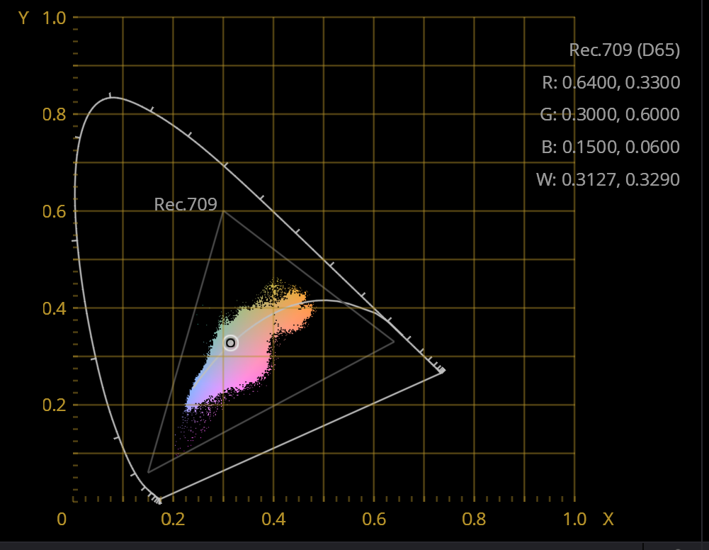
@PM490 Hi Pablo, there is a nice walk-through with respects to the steps involved at Jack Hogan’s blog. He goes into much more detail. However, here’s a short python script which shows some possiblities. You should download the following raw file, “xp24_full.dng” for the script. It was captured by the HQ sensor.
Any .dng-file is in reality a special .tif-file with some additional tags. In the following script, I show you two ways to access the data hidden in the .dng-file: either rawpy or exifread. rawpy is in fact an interface to libraw and could be used to do it all at conce - that is, develop your raw file directly into a nice image. I am using rawpy here only to access certain original data and I am doing the processing by myself. You could instead use exifread or your own software to do so.
Anyway, here’s the full script which should work out of the box, once you have installed the necessary libraries: cv2, numpy, rawpy and exifread. I will go through each line of code in the following:
import cv2
import numpy as np

import rawpy
import exifread

path = r'G:\xp24_full.dng'

# utility fct for zooming in
def showCutOut(title,data,scale=1,norm=True):

    x0   = 1100
    y0   = 1600
    size = 1024

    x0   //= scale
    y0   //= scale
    size //= scale

    cutOut = data[ y0: y0+size, x0: x0+size].astype(np.float32)
    if norm:
        cutOut = (0xffff*(cutOut - cutOut.min())/(cutOut.max() - cutOut.min())).astype(np.uint16)

    # minor cosmetic cleanup
    img_bgr = cv2.cvtColor(cutOut, cv2.COLOR_RGB2BGR)
    cv2.imshow(title,img_bgr)
    cv2.waitKey(500)

# opening the raw image file
rawfile = rawpy.imread(path)

# get the raw bayer
bayer_raw = rawfile.raw_image_visible

# check the basic data we got
print('DataType: ',bayer_raw.dtype)
print('Shape   : ',bayer_raw.shape)
print('Minimum : ',bayer_raw.min())
print('Maximum : ',bayer_raw.max())

# grap an interesting part out of the raw data and show it
showCutOut("Sensor Data",bayer_raw)

# quick-and-dirty debayer
if rawfile.raw_pattern[0][0]==2:

    # this is for the HQ camera
    red    =  bayer_raw[1::2, 1::2].astype(np.float32)                                 # Red
    green1 =  bayer_raw[0::2, 1::2].astype(np.float32)                                 # Gr/Green1
    green2 =  bayer_raw[1::2, 0::2].astype(np.float32)                                 # Gb/Green2
    blue   =  bayer_raw[0::2, 0::2].astype(np.float32)                                 # Blue

elif rawfile.raw_pattern[0][0]==0:

    # ... and this one for the Canon 70D, IXUS 110 IS, Canon EOS 1100D, Nikon D850
    red    =  bayer_raw[0::2, 0::2].astype(np.float32)                                 # Red
    green1 =  bayer_raw[0::2, 1::2].astype(np.float32)                                 # Gr/Green1
    green2 =  bayer_raw[1::2, 0::2].astype(np.float32)                                 # Gb/Green2
    blue   =  bayer_raw[1::2, 1::2].astype(np.float32)                                 # Blue

elif rawfile.raw_pattern[0][0]==1:

    # ... and this one for the Sony
    red    =  bayer_raw[0::2, 1::2].astype(np.float32)                                 # red
    green1 =  bayer_raw[0::2, 0::2].astype(np.float32)                                 # Gr/Green1
    green2 =  bayer_raw[1::2, 1::2].astype(np.float32)                                 # Gb/Green2
    blue   =  bayer_raw[1::2, 0::2].astype(np.float32)                                 # blue

else:
    print('Unknown filter array encountered!!')

# creating the raw RGB
camera_raw_RGB = np.dstack( [1.0*red,(1.0*green1+green2)/2,1.0*blue] )
showCutOut("Camera Raw",camera_raw_RGB,2)

# getting the black- and whitelevels
blacklevel   = np.average(rawfile.black_level_per_channel)
whitelevel   = rawfile.white_level

# get the WP
whitebalance = rawfile.camera_whitebalance[0:-1]
whitePoint   = whitebalance / np.amin(whitebalance)

# transforming raw image to normalized raw (with appropriate clipping)
camera_raw_RGB_normalized = np.clip( ( camera_raw_RGB - blacklevel ) / (whitelevel-blacklevel), 0.0, 1.0/whitePoint )

# applying the "As Shot Neutral" whitepoint
scene      = camera_raw_RGB_normalized @ np.diag(whitePoint).T
showCutOut("Scene",scene,2)

# get the ccm from camera
with open(path,'br') as f:
    tags = exifread.process_file(f)
    colorMatrix1 = np.zeros([3,3])
    if 'Image Tag 0xC621' in tags.keys():
        index = 0
        for x in range(0,3):
            for y in range(0,3):
                colorMatrix1[x][y] = float(tags['Image Tag 0xC621'].values[index])
                index = index +1

# http://www.brucelindbloom.com/index.html?Eqn_RGB_XYZ_Matrix.html sRGB D65 -> XYZ
wp_D50_to_D65  = [[0.4124564,  0.3575761,  0.1804375],
                  [0.2126729,  0.7151522,  0.0721750],
                  [0.0193339,  0.1191920,  0.9503041]]

# the matrix taking us from sRGB(linear) to camera RGB, white points adjusting (camera is D50, sRGB is D65)
sRGB_to_camRGB_wb   = colorMatrix1 @ wp_D50_to_D65

# normalizing the matrix in order to avoid color shifts - important!!!
colorMatrix_wb_mult = np.sum(sRGB_to_camRGB_wb, axis=1)
sRGB_to_camRGB      = sRGB_to_camRGB_wb / colorMatrix_wb_mult[:, None]

# finally solving for the inverted matrix, as we want to map from camera RGB to sRGB(linear)
camRGB_to_sRGB      = np.linalg.pinv(sRGB_to_camRGB)

# and we obtain the image in linear RGB
img = scene @ camRGB_to_sRGB.T
showCutOut("Image",img,2,norm=False)

# finally, apply the gamma-curve to the image
rec709 = img
i = rec709 < 0.0031308
j = np.logical_not(i)
rec709[i] = 323 / 25  * rec709[i]
rec709[j] = 211 / 200 * rec709[j] ** (5 / 12) - 11 / 200
showCutOut("rec709",rec709,2,norm=False)
Ok, let’s start. In the beginning, the necessary libs are loaded and the path to our source file is specified:
import cv2
import numpy as np

import rawpy
import exifread

path = r'G:\xp24_full.dng'
Obviously, the later has to be adapted to your needs. A tiny display routine follows - it’s just a quick hack to show you the different processing stages:
# utility fct for zooming in
def showCutOut(title,data,scale=1,norm=True):

    x0   = 1100
    y0   = 1600
    size = 1024

    x0   //= scale
    y0   //= scale
    size //= scale

    cutOut = data[ y0: y0+size, x0: x0+size].astype(np.float32)
    if norm:
        cutOut = (0xffff*(cutOut - cutOut.min())/(cutOut.max() - cutOut.min())).astype(np.uint16)

    # minor cosmetic cleanup
    img_bgr = cv2.cvtColor(cutOut, cv2.COLOR_RGB2BGR)
    cv2.imshow(title,img_bgr)
    cv2.waitKey(500)
I am using different means of displaying my data. Anyway, opening a raw file with python is as easy as
# opening the raw image file
rawfile = rawpy.imread(path)

# get the raw bayer
bayer_raw = rawfile.raw_image_visible
Note that at that point, you’d be in a position to develop the raw with all the fancy stuff libraw/rawpy is offering, but that is not our aim here. Let’s see what data we actually got:
# check the basic data we got
print('DataType: ',bayer_raw.dtype)
print('Shape : ',bayer_raw.shape)
print('Minimum : ',bayer_raw.min())
print('Maximum : ',bayer_raw.max())
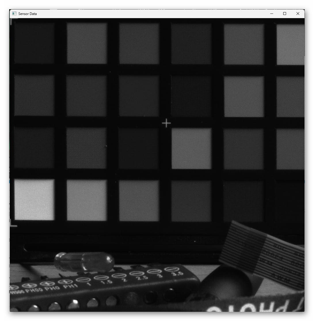
# grap an interesting part out of the raw data and show it
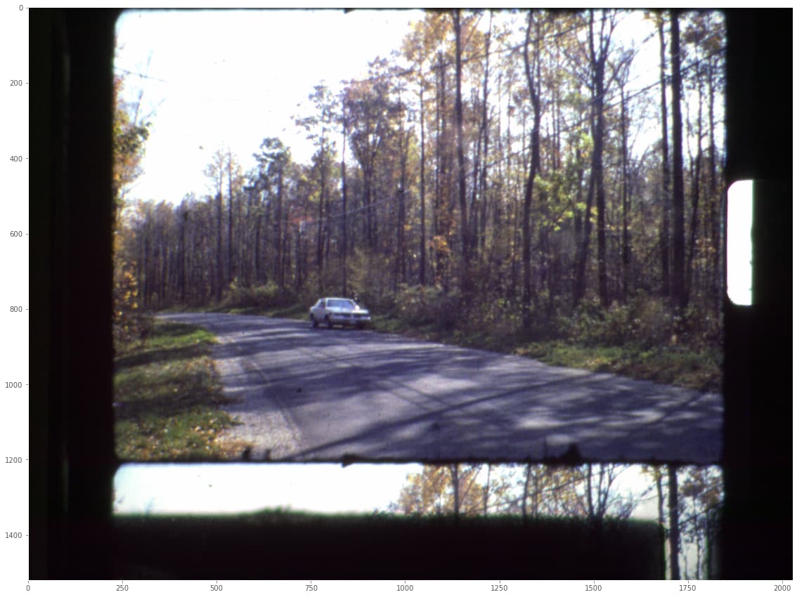
showCutOut("Sensor Data",bayer_raw)
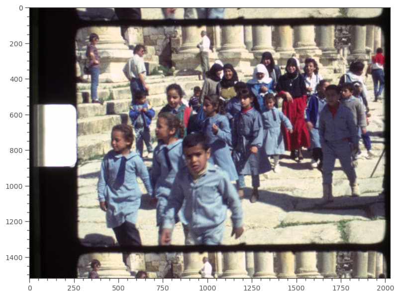
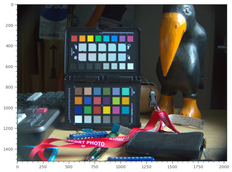
You should see something like that:
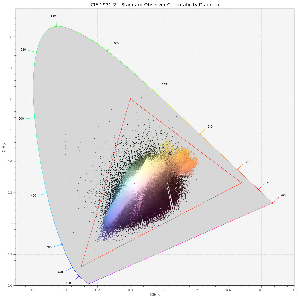
That is the raw Bayer-pattern. If you zoom in appropriately, you are going to see different gray patterns in each of the color patches. That’s how your sensor is encoding different colors.
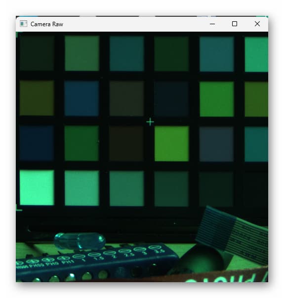
Debayering is an art, and libraw/pyraw can do this for you. As I am not interested in full-res imagery here (only for analysis I develop on my own), I employ the simplest debayer possible:
# quick-and-dirty debayer
if rawfile.raw_pattern[0][0]==2:

    # this is for the HQ camera
    red    =  bayer_raw[1::2, 1::2].astype(np.float32)                                 # Red
    green1 =  bayer_raw[0::2, 1::2].astype(np.float32)                                 # Gr/Green1
    green2 =  bayer_raw[1::2, 0::2].astype(np.float32)                                 # Gb/Green2
    blue   =  bayer_raw[0::2, 0::2].astype(np.float32)                                 # Blue

elif rawfile.raw_pattern[0][0]==0:

    # ... and this one for the Canon 70D, IXUS 110 IS, Canon EOS 1100D, Nikon D850
    red    =  bayer_raw[0::2, 0::2].astype(np.float32)                                 # Red
    green1 =  bayer_raw[0::2, 1::2].astype(np.float32)                                 # Gr/Green1
    green2 =  bayer_raw[1::2, 0::2].astype(np.float32)                                 # Gb/Green2
    blue   =  bayer_raw[1::2, 1::2].astype(np.float32)                                 # Blue

elif rawfile.raw_pattern[0][0]==1:

    # ... and this one for the Sony
    red    =  bayer_raw[0::2, 1::2].astype(np.float32)                                 # red
    green1 =  bayer_raw[0::2, 0::2].astype(np.float32)                                 # Gr/Green1
    green2 =  bayer_raw[1::2, 1::2].astype(np.float32)                                 # Gb/Green2
    blue   =  bayer_raw[1::2, 0::2].astype(np.float32)                                 # blue

else:
    print('Unknown filter array encountered!!')

# creating the raw RGB
camera_raw_RGB = np.dstack( [1.0*red,(1.0*green1+green2)/2,1.0*blue] )
showCutOut("Camera Raw",camera_raw_RGB,2)
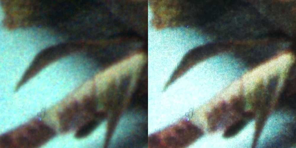
This code section looks at the “raw_pattern” spec in pyraw’s data structure and resamples the full Bayer-pattern into separate color channels, half the size of the original. It than adds the two green channels and stacks all together into a single RGB image. This image looks still weird,
showing the typical green cast of an unprocessed raw.
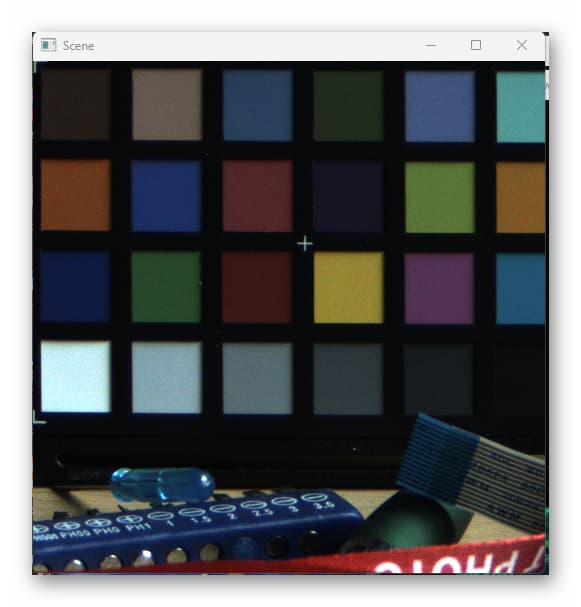
The next processing step is to adjust for black and white levels in the data. Never assume you know which data range is used in your raw - you might be surprised! (For starters, the RP5 stores differently from a RP4, for example.)
# getting the black- and whitelevels
blacklevel   = np.average(rawfile.black_level_per_channel)
whitelevel   = rawfile.white_level

# get the WP
whitebalance = rawfile.camera_whitebalance[0:-1]
whitePoint   = whitebalance / np.amin(whitebalance)

# transforming raw image to normalized raw (with appropriate clipping)
camera_raw_RGB_normalized = np.clip( ( camera_raw_RGB - blacklevel ) / (whitelevel-blacklevel), 0.0, 1.0/whitePoint )

# applying the "As Shot Neutral" whitepoint
scene      = camera_raw_RGB_normalized @ np.diag(whitePoint).T
showCutOut("Scene",scene,2)
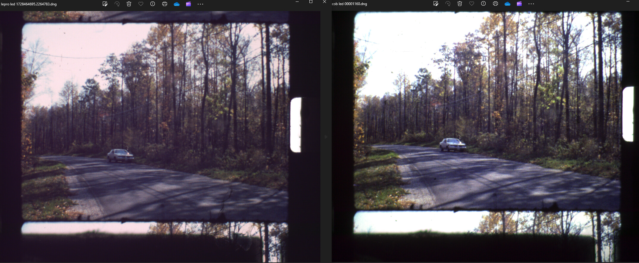
There are several important things happening here. Note the np.clip operation which happens first, using the whitePoint of the raw. This ensures that you do not end up with magenta highlights. More details can be read in Jack Hogan’s blog, linked above. The second step (applying the whitebalance) actually recovers something usable - but we are still far from where we will end up! Here’s the intermediate result:
This is the image in the camera’s RGB space. It is a manufacturer designed color space and needs to be mapped into a RGB space which our display can understand. We’re not there yet.
For this, we have to recover the only color matrix available to us in raw HQ sensor data. I am using here, just for the fun of it, the exifread library. As you will notice, it’s much less convient than the rawpy one - for starters, you will need to know the image tag you are after:
# get the ccm from camera_
with open(path,'br') as f:
    tags = exifread.process_file(f)
    colorMatrix1 = np.zeros([3,3])
    if 'Image Tag 0xC621' in tags.keys():
        index = 0
        for x in range(0,3):
            for y in range(0,3):
                colorMatrix1[x][y] = float(tags['Image Tag 0xC621'].values[index])
                index = index +1
Anyway. Once we have that matrix, we need to do some additional matrix calculations. There are two main reasons: first, the matrix we get from the .dng is mapping into the wrong whitepoint (D50). So we need to throw in an adjustment matrix. Secondly, the mapping is the wrong way around. So we need to invert the mapping. In addition, we need to take care that the transformation we are about to calculate is proper normalized. All this is handled here:
# http://www.brucelindbloom.com/index.html?Eqn_RGB_XYZ_Matrix.html sRGB D65 -> XYZ
wp_D50_to_D65 = [[0.4124564, 0.3575761, 0.1804375],
[0.2126729, 0.7151522, 0.0721750],
[0.0193339, 0.1191920, 0.9503041]]
# the matrix taking us from sRGB(linear) to camera RGB, white points adjusting (camera is D50, sRGB is D65)
sRGB_to_camRGB_wb = colorMatrix1 @ wp_D50_to_D65
# normalizing the matrix in order to avoid color shifts - important!!!
colorMatrix_wb_mult = np.sum(sRGB_to_camRGB_wb, axis=1)
sRGB_to_camRGB = sRGB_to_camRGB_wb / colorMatrix_wb_mult[:, None]
# finally solving for the inverted matrix, as we want to map from camera RGB to sRGB(linear)
camRGB_to_sRGB = np.linalg.pinv(sRGB_to_camRGB)
# and we obtain the image in linear RGB
img = scene @ camRGB_to_sRGB.T
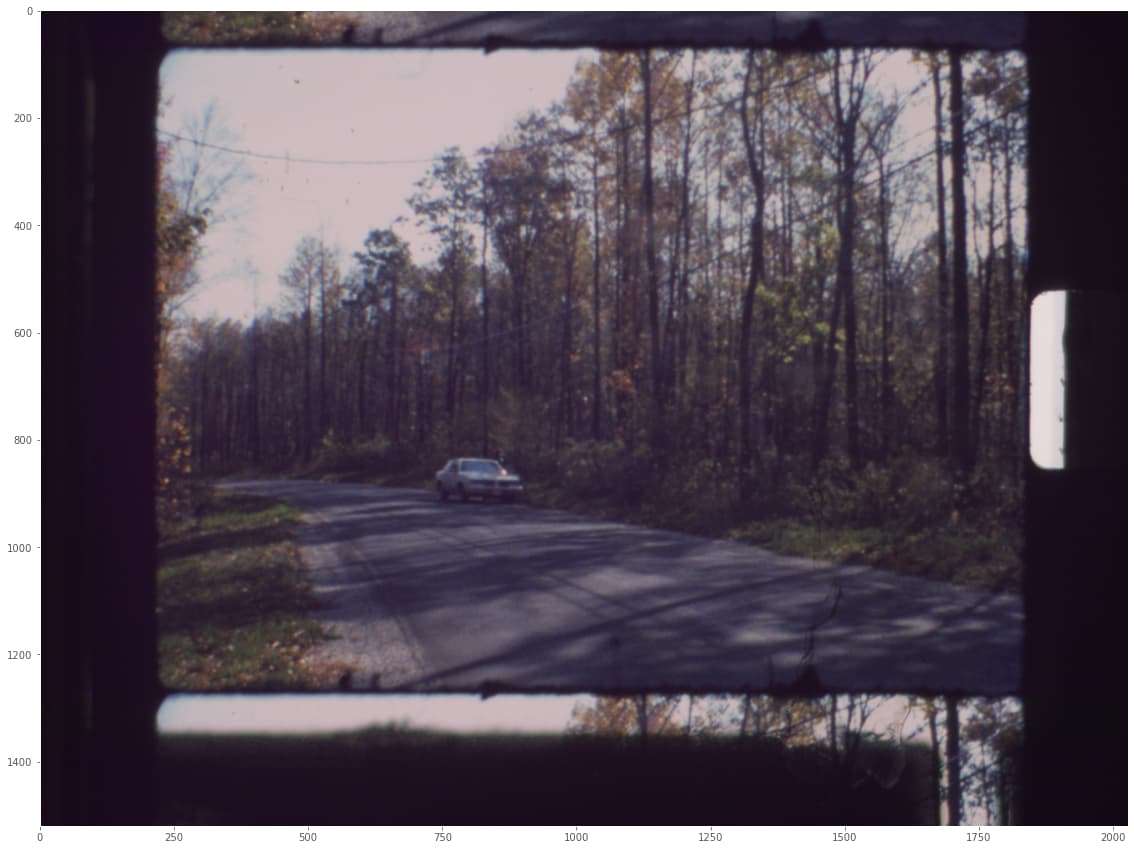
showCutOut("Image",img,2,norm=False)
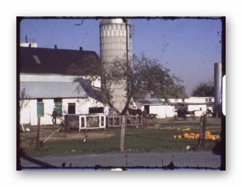
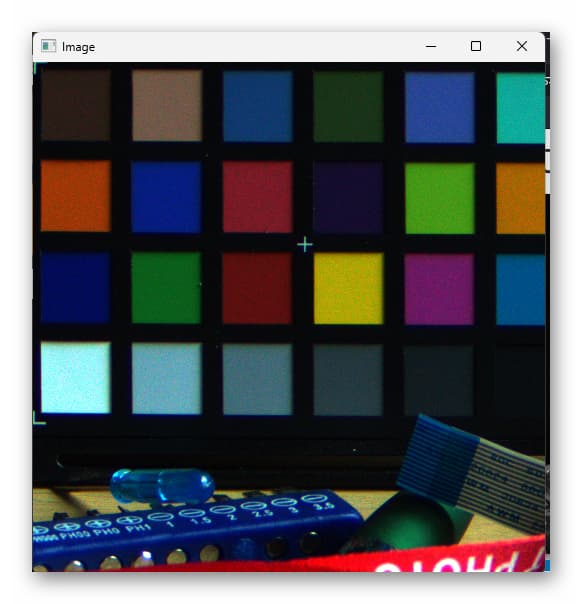
We should end up with the following image:
Well, that thing looks aweful, right? What is happening? Now, this is the image data with
linear RGB-values, and that is not what your display is actually expecting. In a final step, we need to appy the appropriate gamma-curve to this data:
# finally, apply the gamma-curve to the image
rec709 = img
i = rec709 < 0.0031308
j = np.logical_not(i)
rec709[i] = 323 / 25 * rec709[i]
rec709[j] = 211 / 200 * rec709[j] ** (5 / 12) - 11 / 200
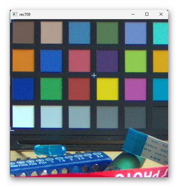
showCutOut("rec709",rec709,2,norm=False)
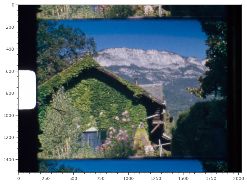
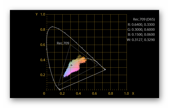
and we end up with this:
– which seems to be ok.
Whether the pipeline I described above is a correct pipeline - frankly, I do not know. I came up with this way of processing years ago and never bothered to check again, as I was getting similar results as other raw development programs or as DaVinci. Besides, the script above was collected from old work and might contain errors I overlooked - but it should get you started for your own experiments. Again, Jack Hogan’s blog is also a very good resource I highly recommend.