SnailScanToo or 2

[PM490]

Building the Sphere
Previously I shared the findings (failures) on the first round of the SnailScan.

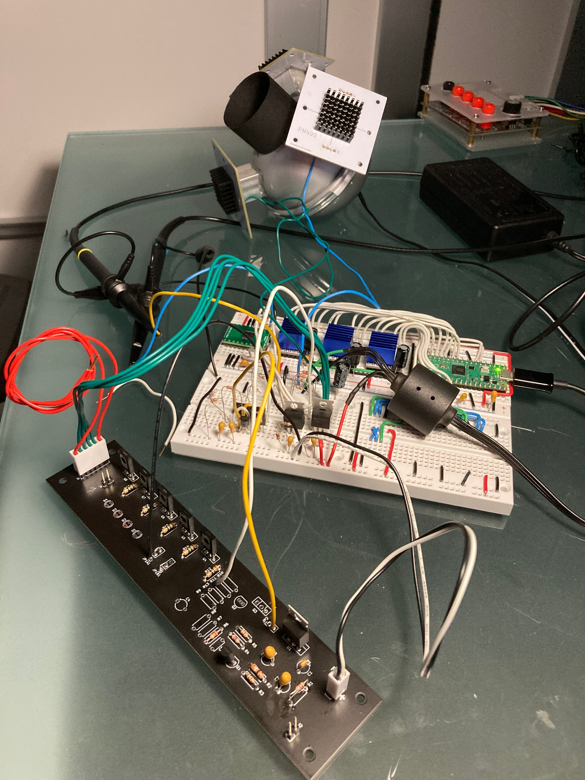
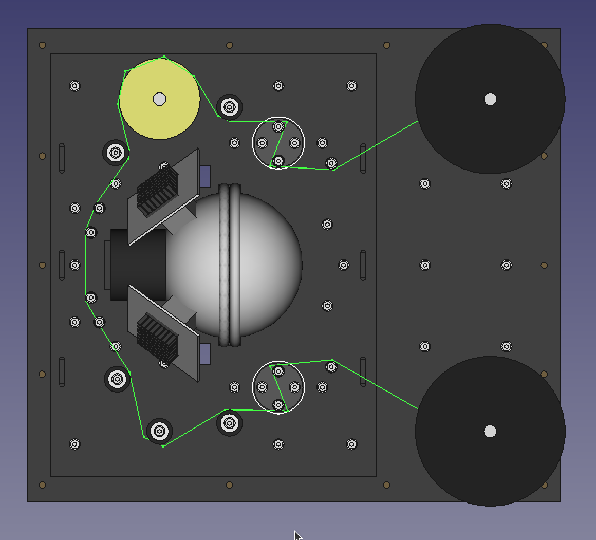
Have been progressing mostly on design choices, and began Frankensteining as much as possible into a prototype, first on the transport, now on the illuminant. The goal is to button up as much as possible before the next round of PCBing and metal cutting.

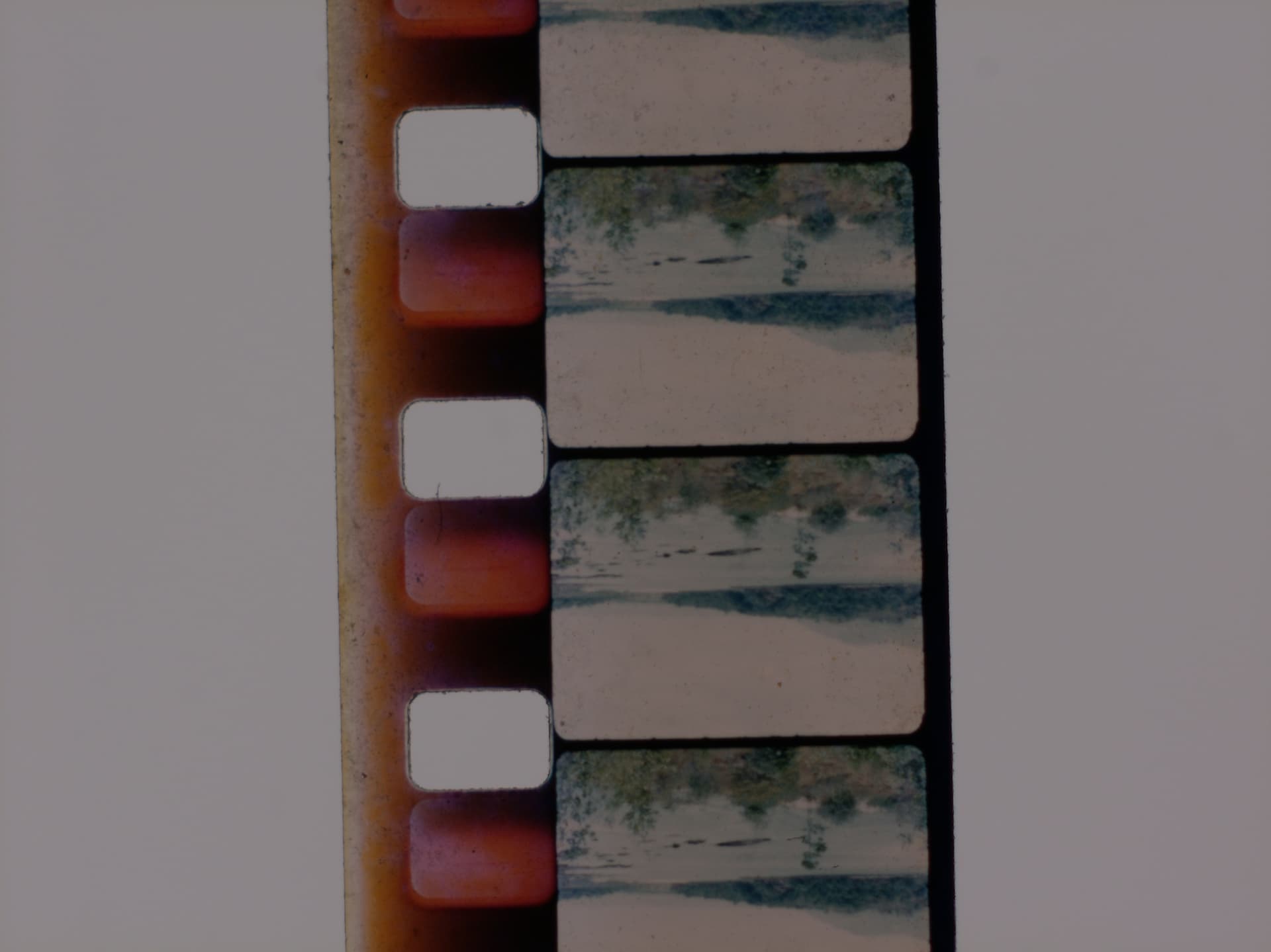
In Snailscan2 the plan was to build a larger sphere to accommodate, at the minimum, about 3 frames of 16 mm.

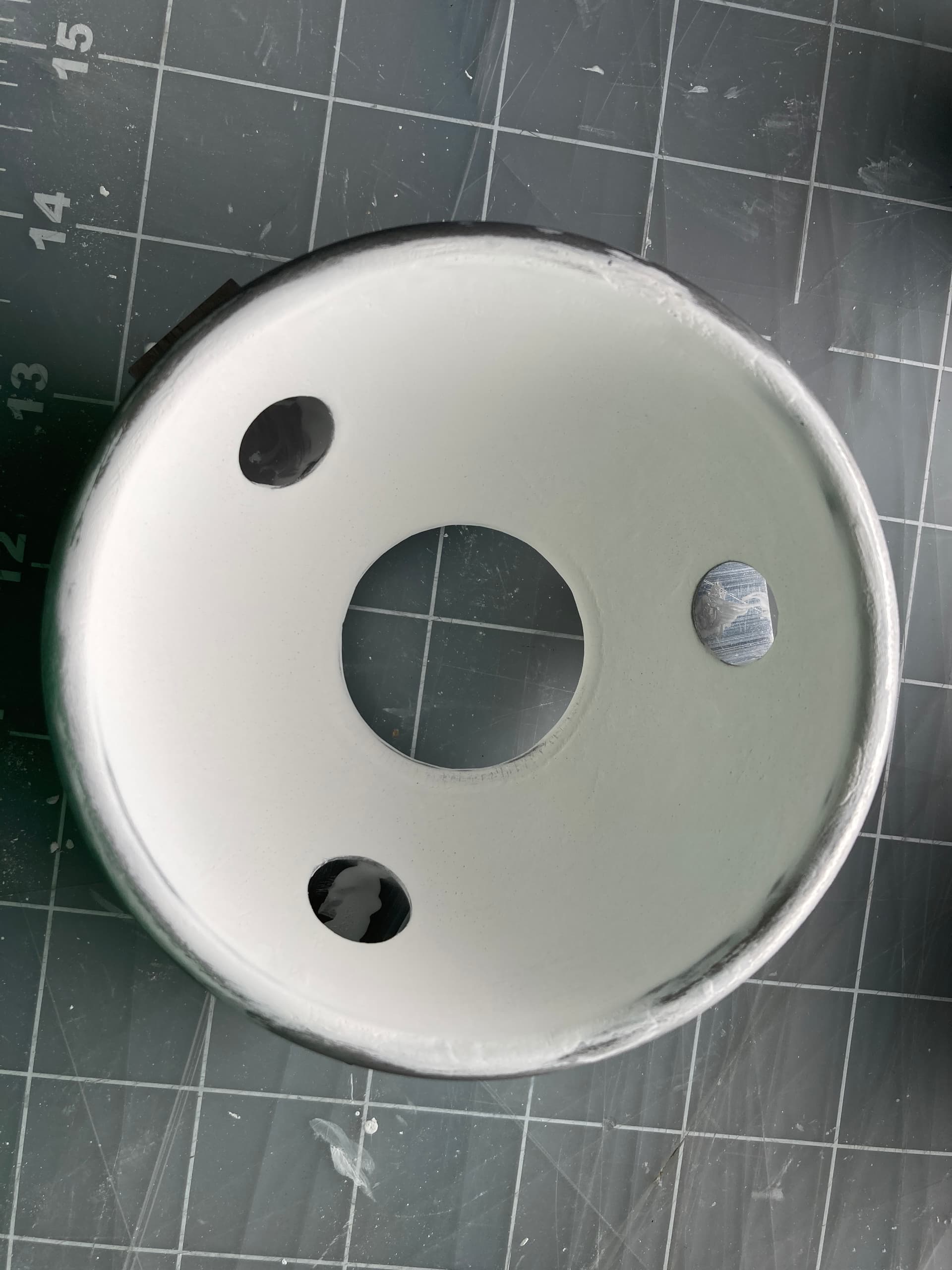
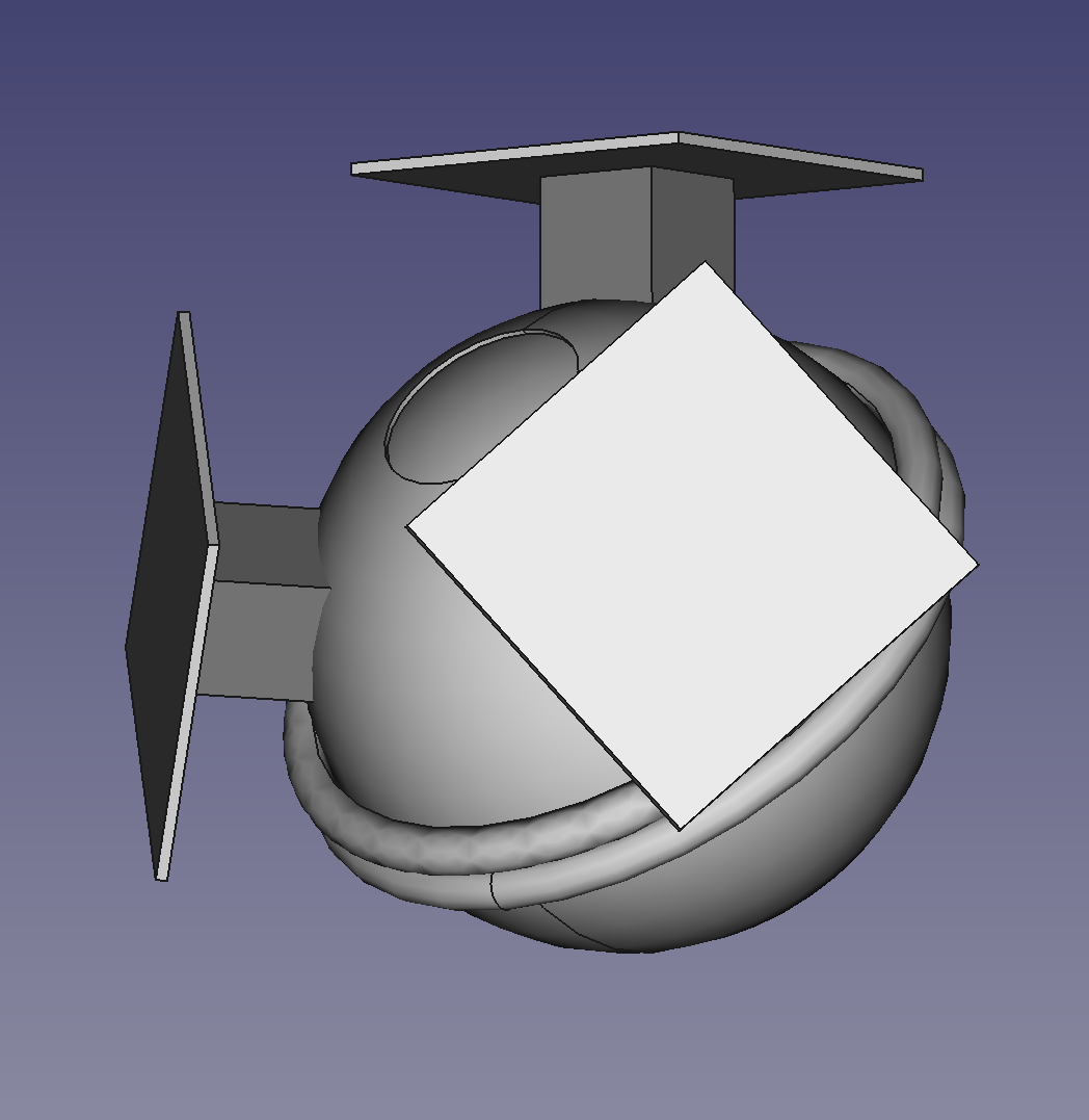
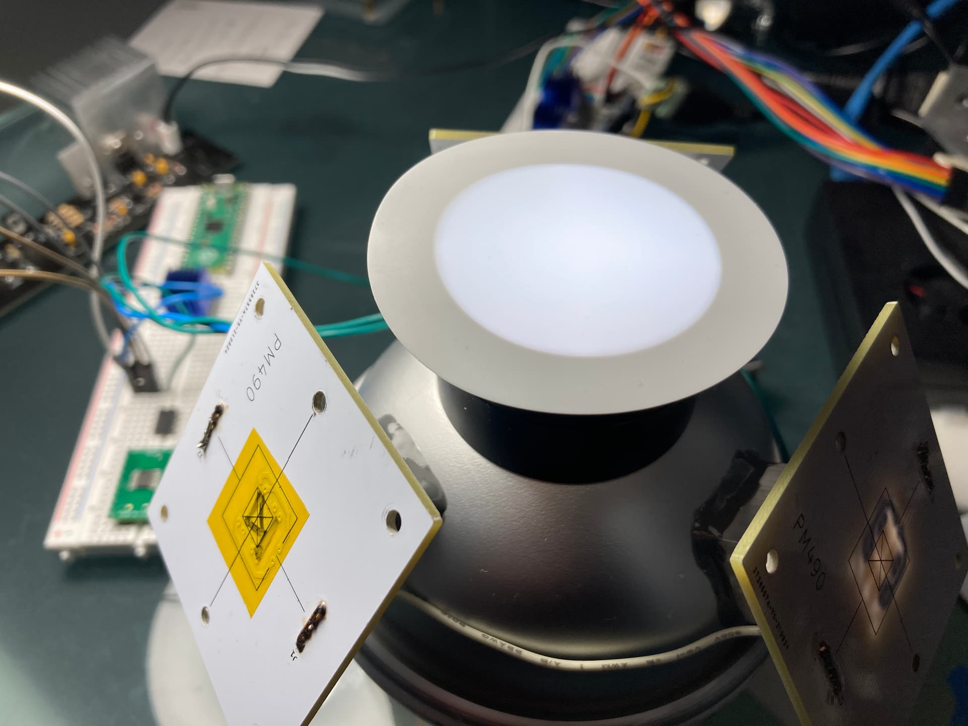
In reply to other postings, I have commented about the half-sphere aluminum baking mold as an option. The sphere was build using the hemisphere aluminum baking molds (90mm diameter). On one half, 3 round entry ports (12 mm diameter) were drilled with a step-bit, and one large output port was cut (39mm diameter). The entry ports were extended with 3/4-inch aluminum square tube epoxy-welded to the sphere-half. The finished part were sanded with a 200 grit paper, and painted with multiple coats of a mixture barium sulfate diluted in distilled water, mixed with acrylic white paint.

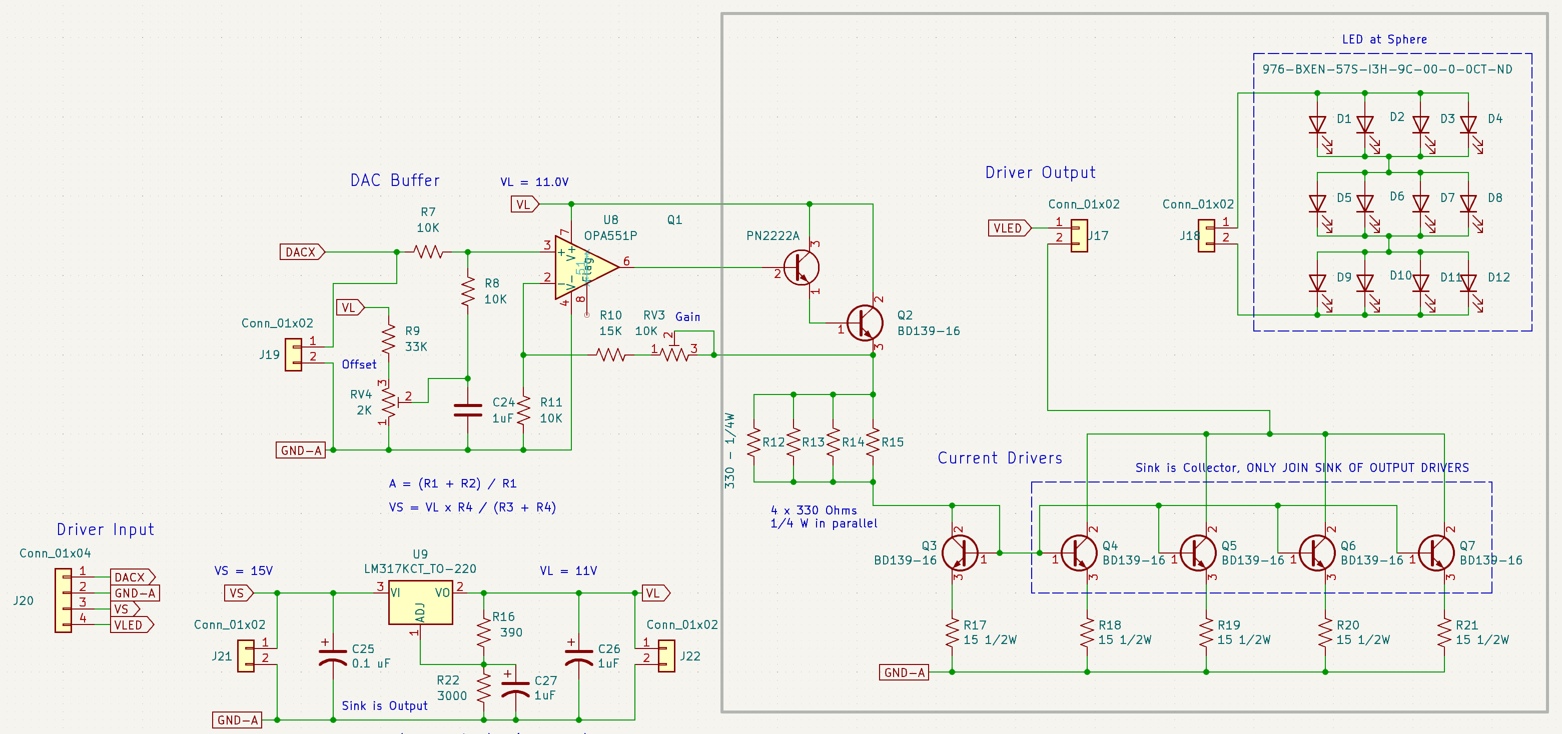
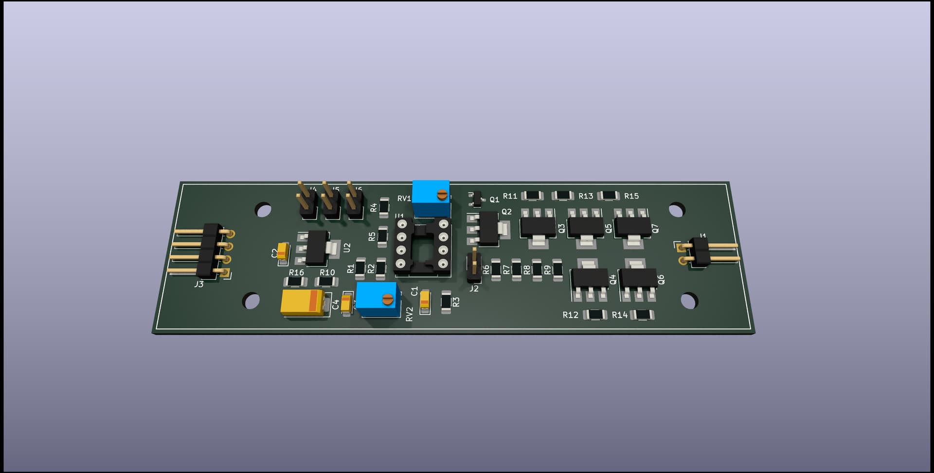
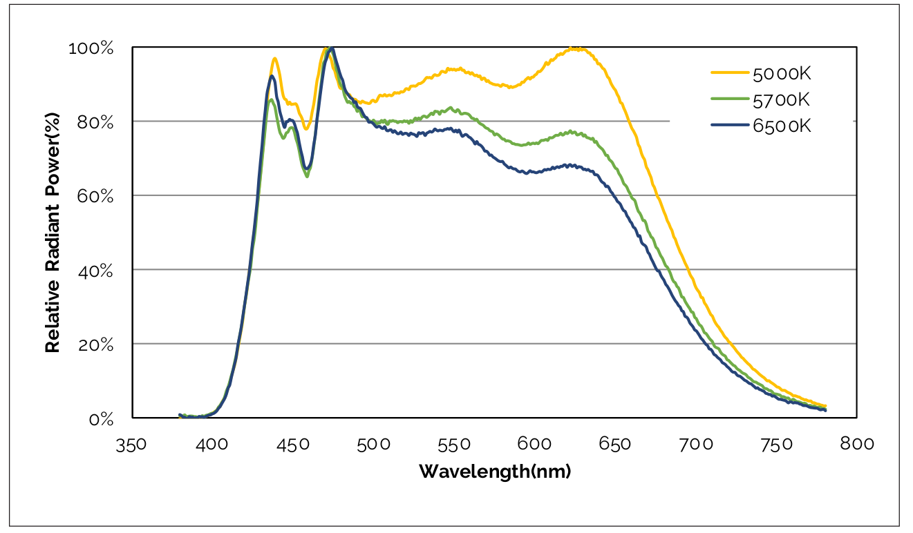
The prototype uses prior-design-existing LED PCBs, and the part of the constant-current driver previously shared. Each PCB has four LEDs, each LED is driven at about 0.7 watts. The LEDs are rated with a CRI>95, see the 5000K curve.

Plenty of light, and too much to use continuously at full power (unless baking something).

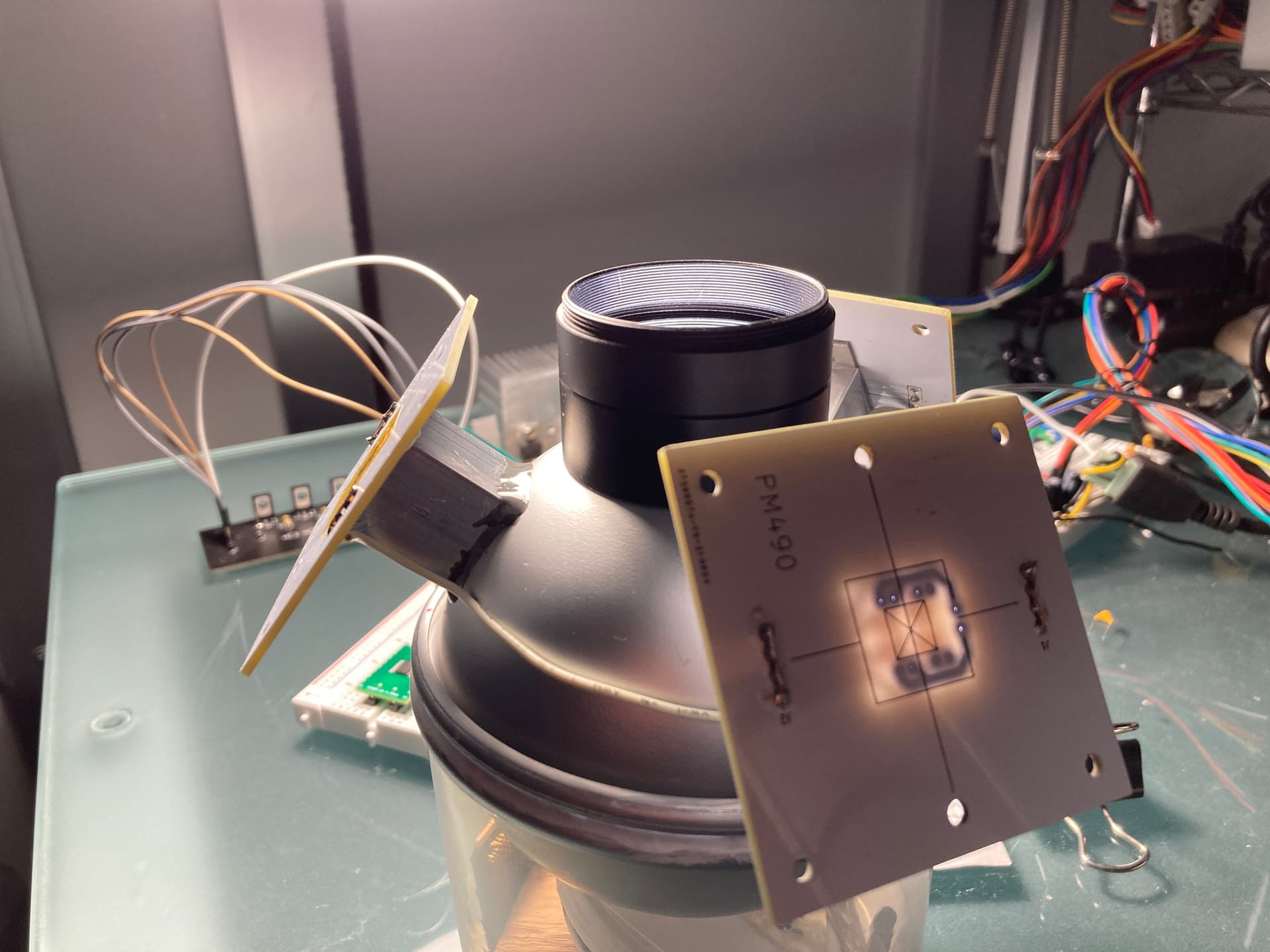
Since I had the existing LED boards, the prototype would require a connector cylinder from the sphere to the gate to avoid spilling it everywhere. The separation, makes clear that the distance between the film, and the sphere surface, has important implications: the intensity and cohesion of the light changes slightly.

Most of the spheres in the forum keep the film close to the sphere, and -if my interpretation is correct- that also provides more-diffuse less-coherent light. When the output port is separated, the same light comes out, but the cylinder somewhat narrows it, making it a bit more-coherent less-diffuse than at the surface. This is very subtle.

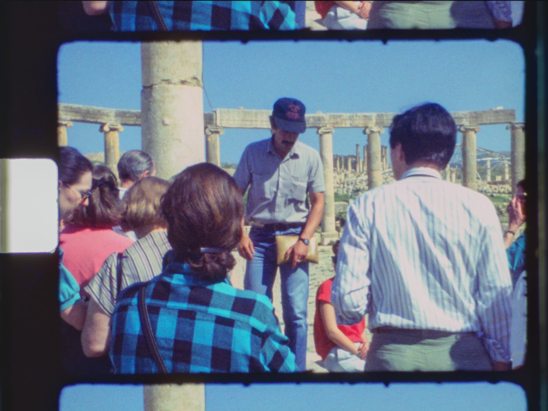
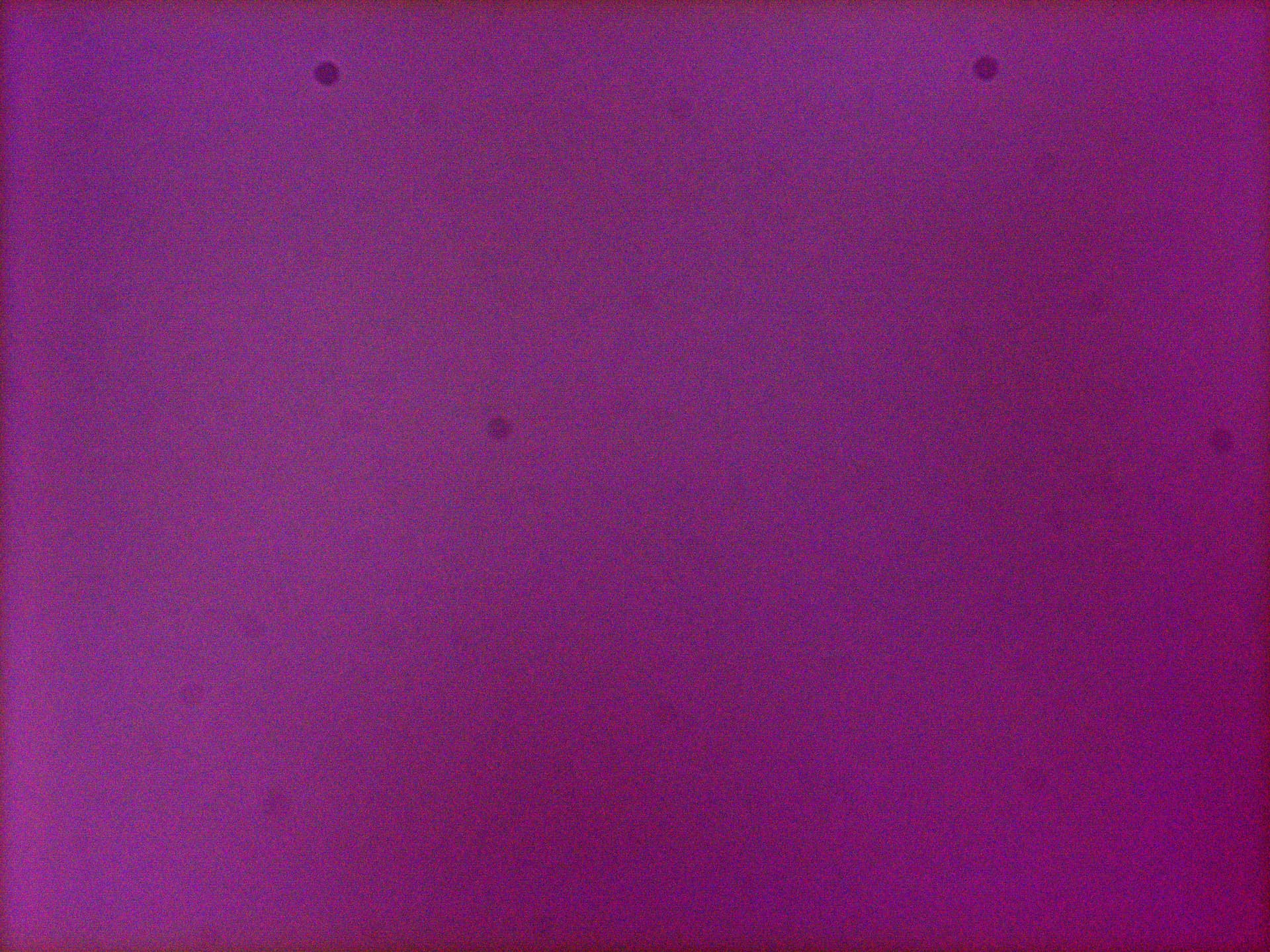
To illustrate, the pictures below have the same LED intensity.
Near the surface:

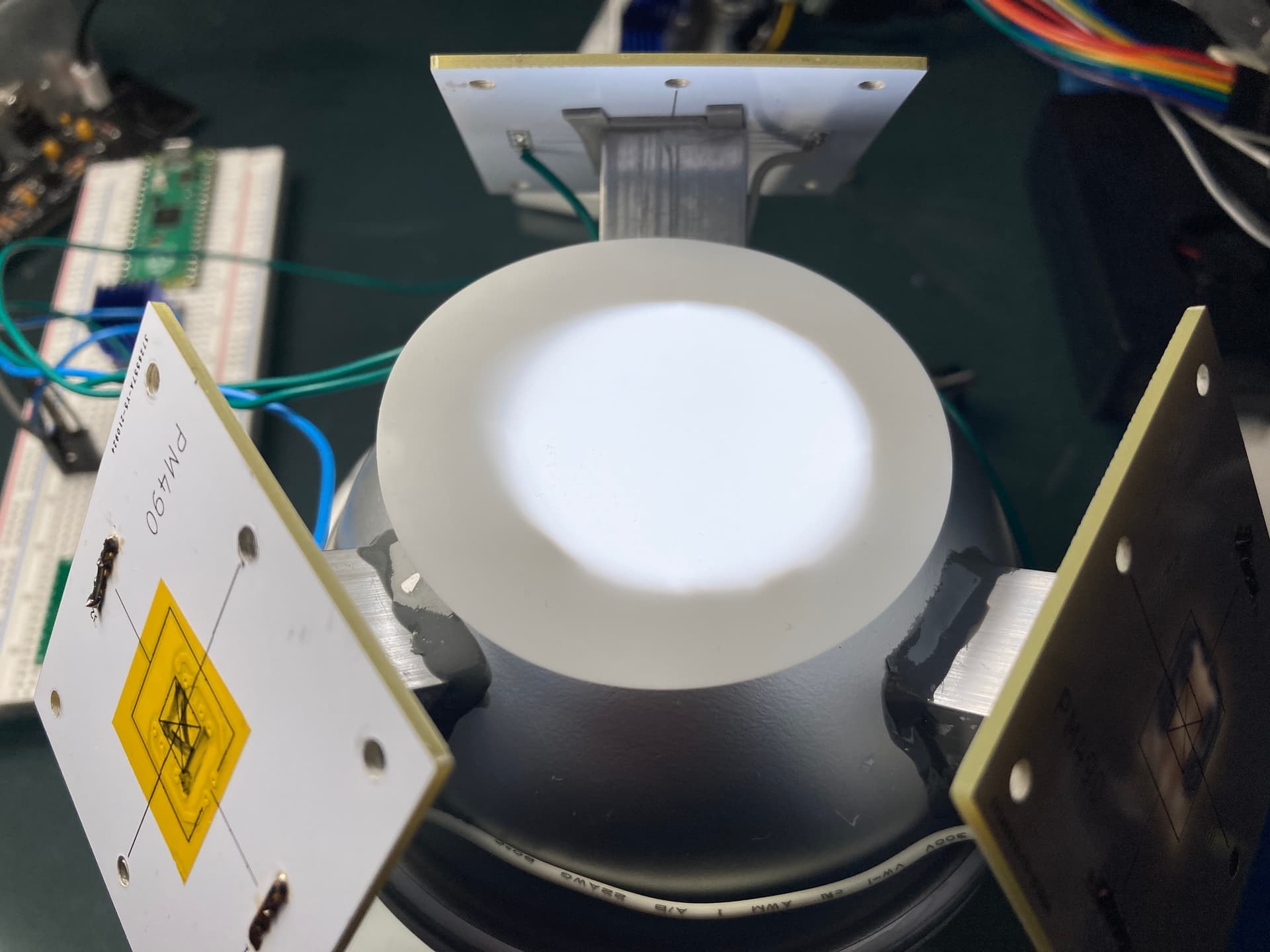
With a 34mm length 42mm diameter extension cylinder:

For me this was an interesting realization, yet something I should have known already: the distance from the film to the sphere surface, slightly changes the nature (diffusion) of the illuminant.

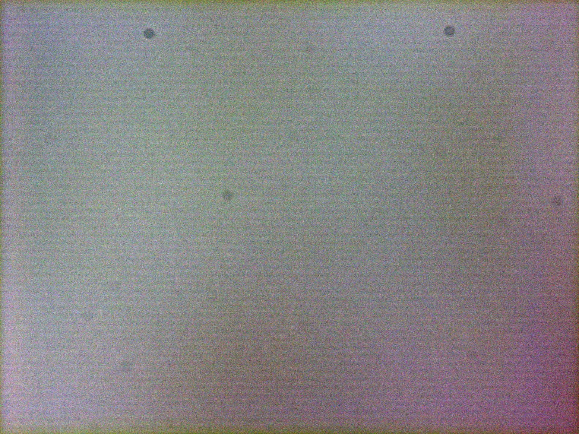
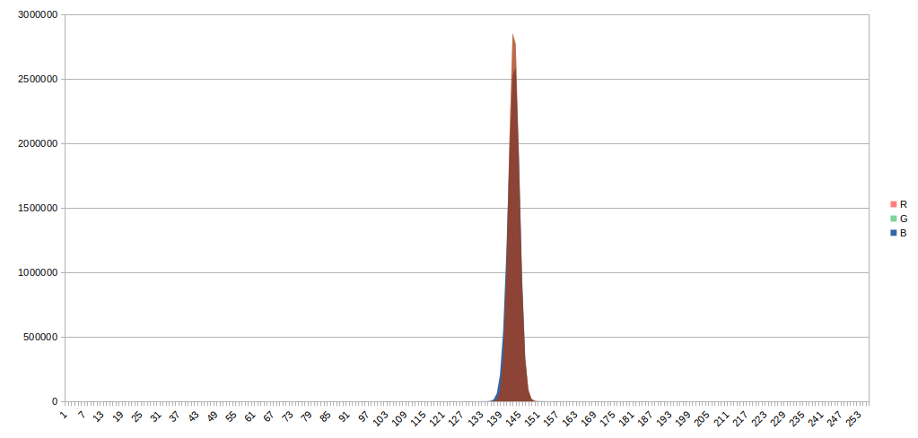
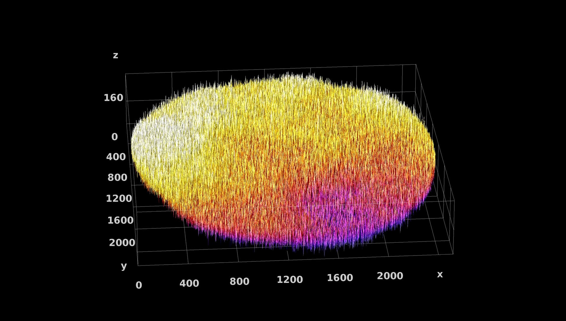
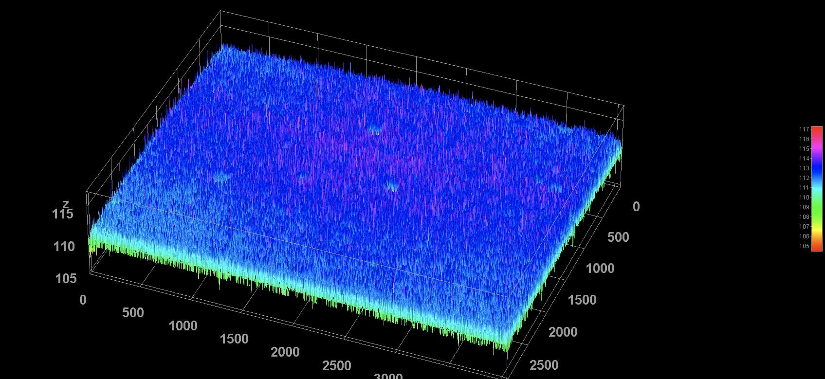
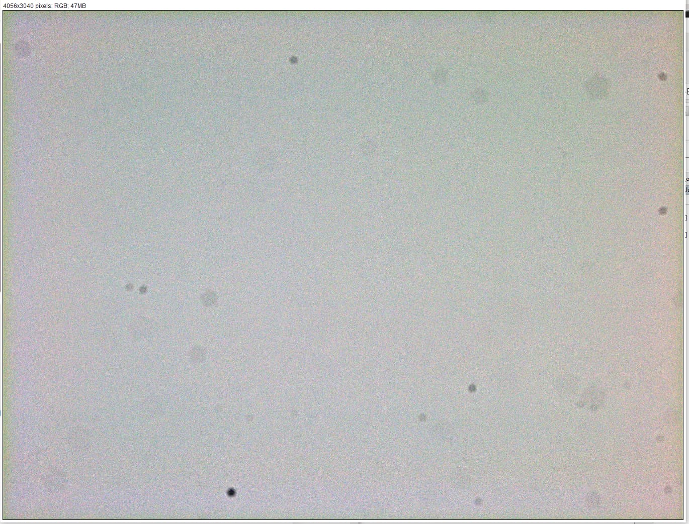
The following takes are with the same parameters, with and without the film. The PNG files were used with ImageJ using the Interactive 3D plugin for the surface plots.

$ libcamera-still --awb=daylight --tuning-file=‘imx477_scientific.json’ --saturation=1 --awbgains=1.65,1.86 --denoise=off --rawfull=1 --mode=4056:3040:12:P --encoding png --raw --n --shutter=1000 --o filename.png

Setup
The test pictures were taken with a Raspberry HQ sensor and Nikkor EL 50mm f2.4 Lens, set between f4 and f5.6. The IR filter of the HQ sensor was removed (had spots) and the setting includes an IR/UV Filter at the front to the lens. The extension tubes and helicoid from the base of the lens to the sensor mount total 54mm.

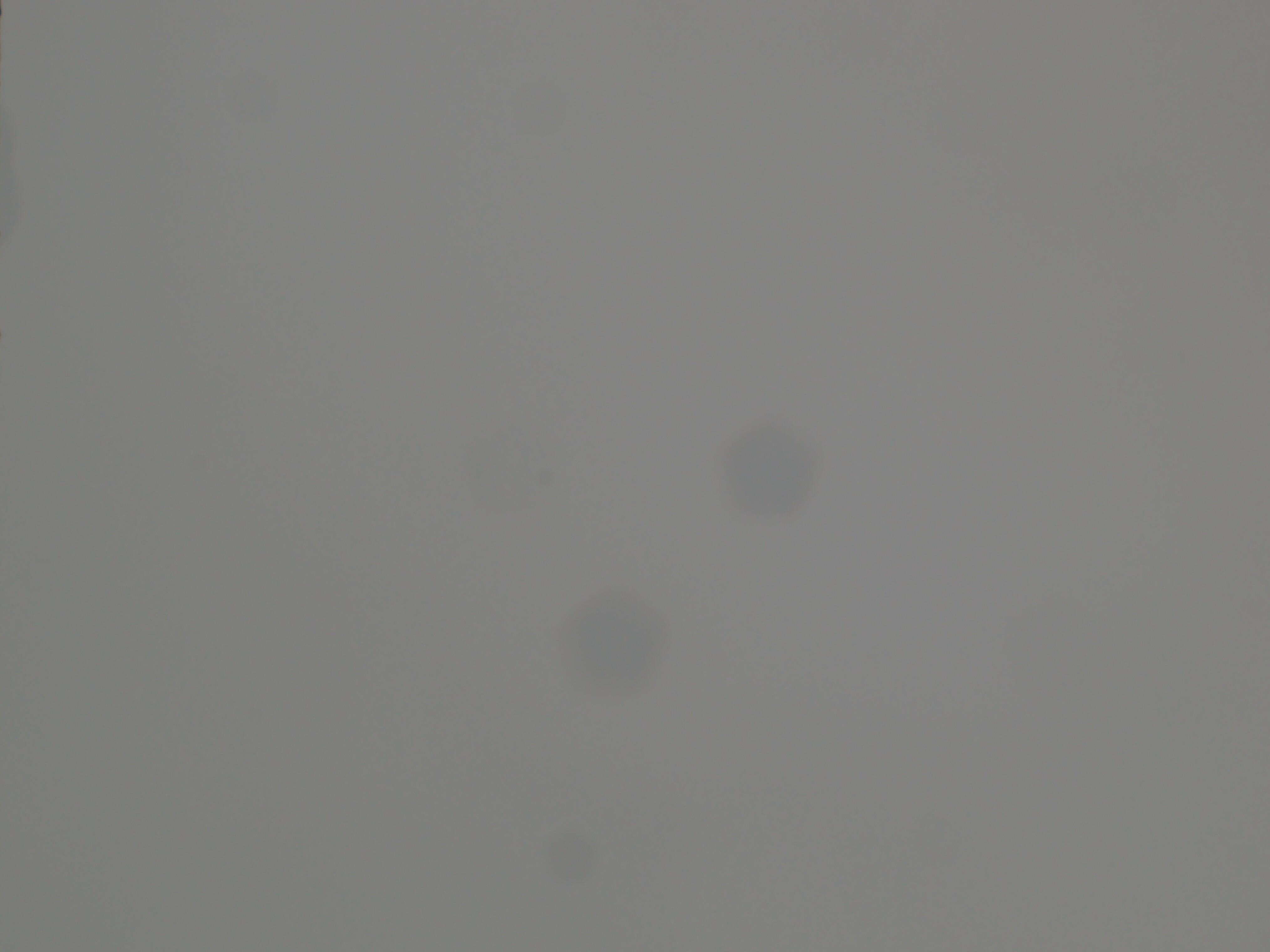
Results

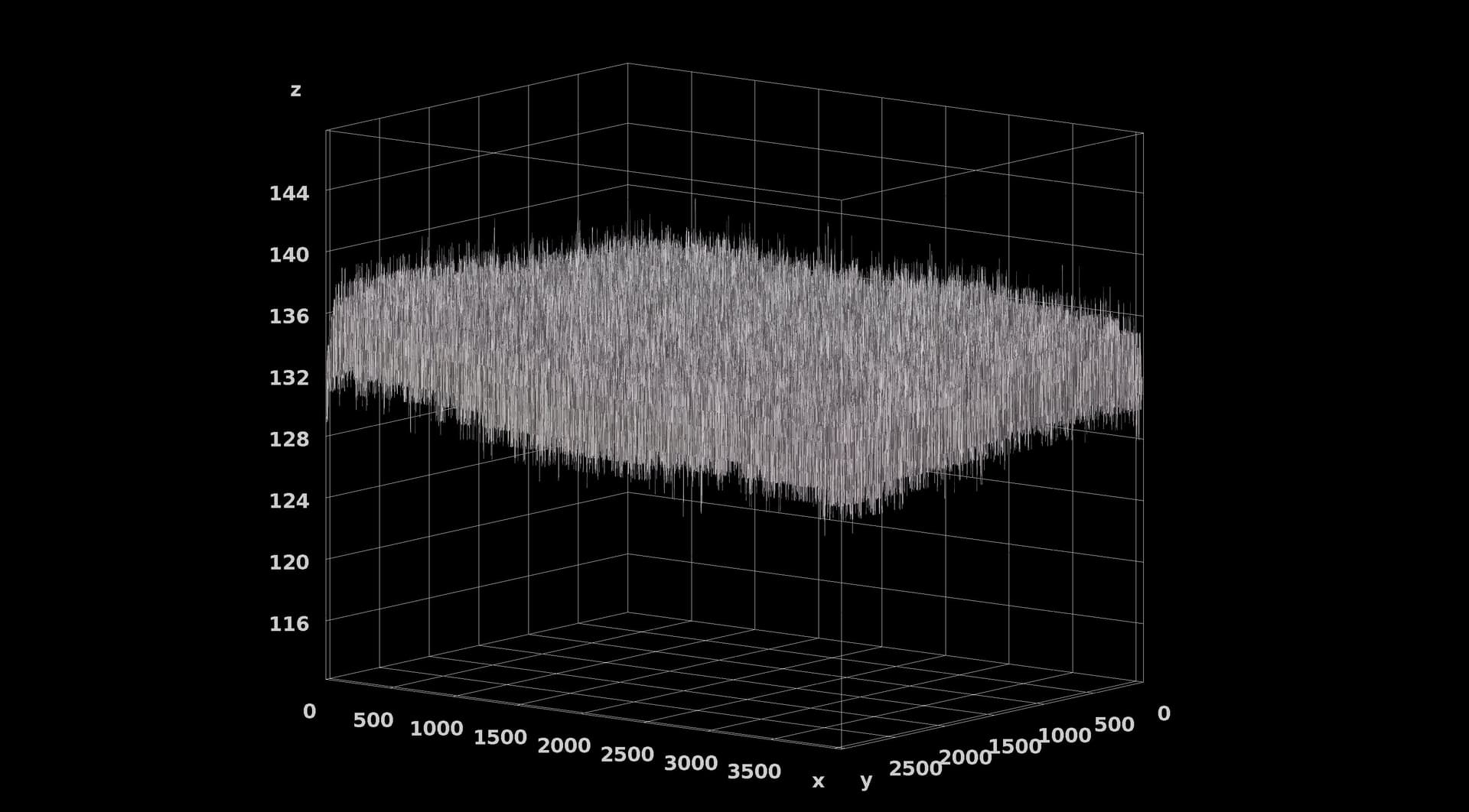
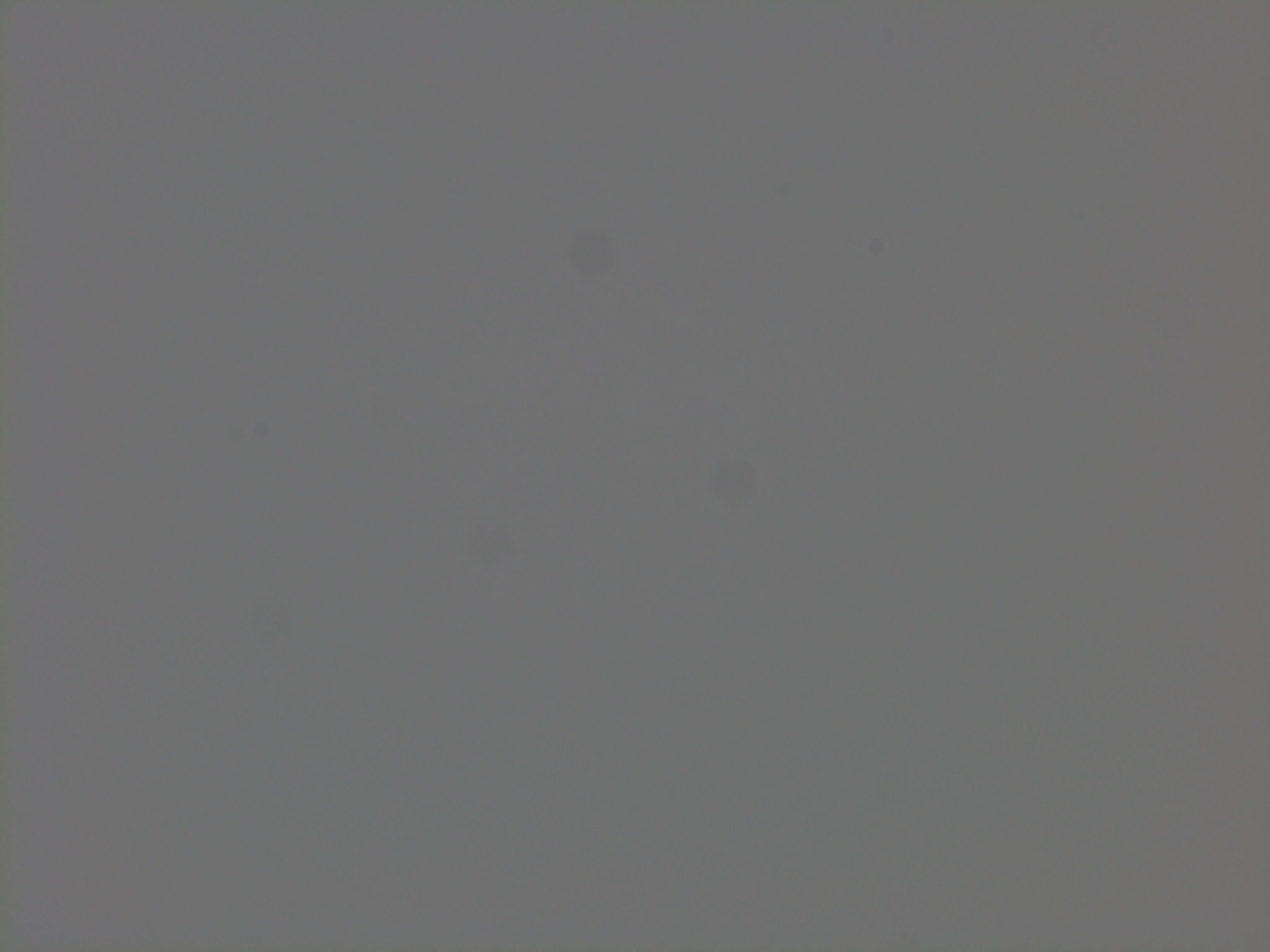
The high-contrast shows a few spsots, these were confirmed (probably dust) to be the sensor.

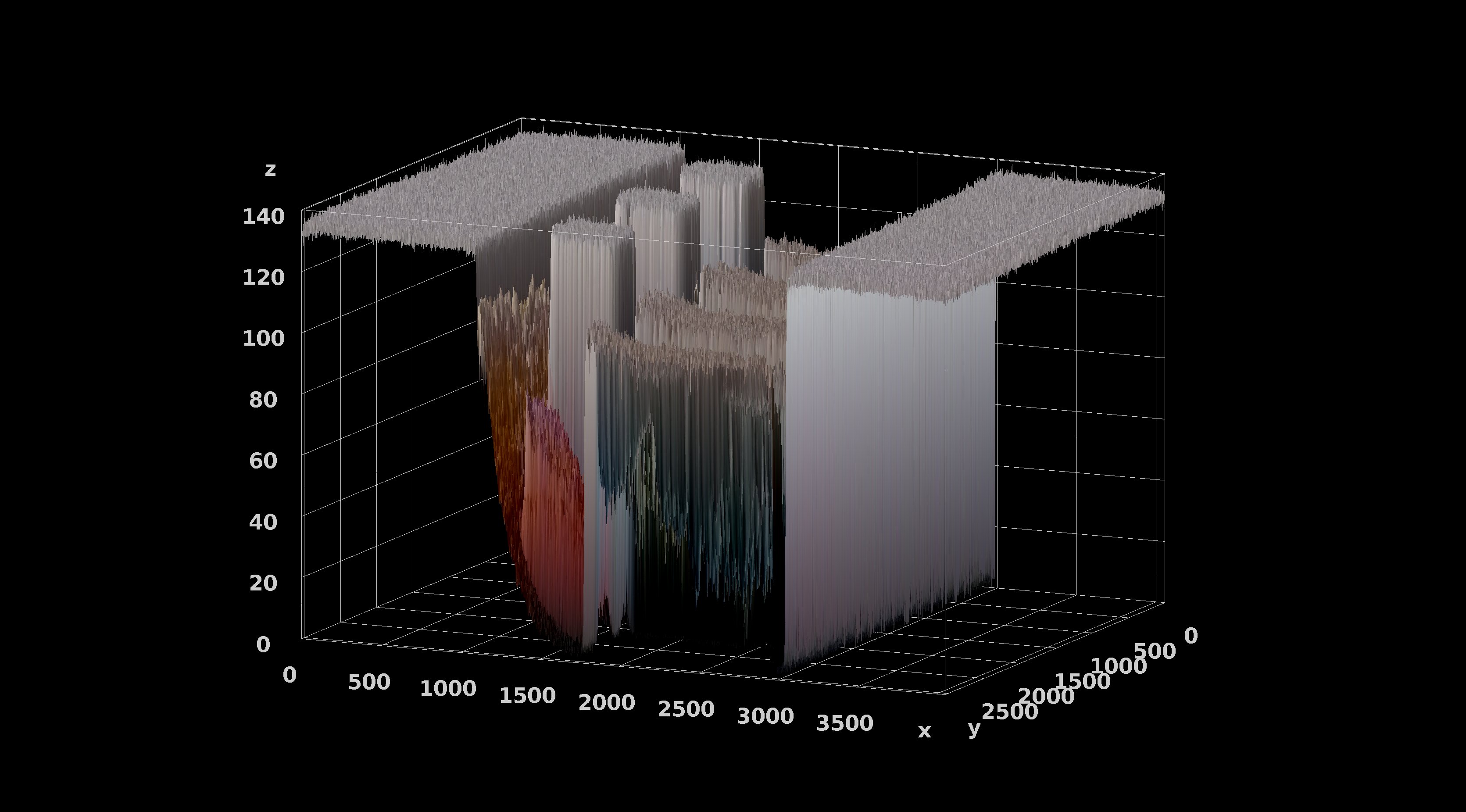
Both surface plots were performed without smoothing on the png file on the plugin of ImageJ.

One important detail of the test setup, and results: only two of the three LED boards on.
It was done to test how well the sphere is performing (and because I need to order some components to change the configuration of the driver to handled all three).

Adding the third will probably not improve the results of the surface plot or histograms, but it would reduce the exposure time.

Conclusions

• Better than expected performance of the sphere for a large output port/sphere diameter.
• Distance from film to sphere makes subtle adjustments in the nature of the illuminant.
• RPi HQ sensor with 2 millisec shutter for normal exposure with about 6 W of white 5000K LED at f4/f5.6.

Special Thanks
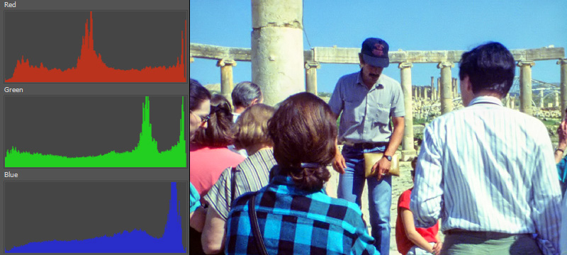
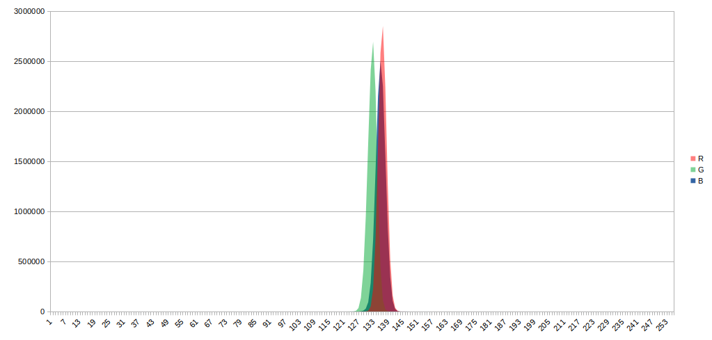
The flatness of this test would not have been possible without the extraordinary work by @cpixip on the color processing of the raspberry new library, and its scientific.json. Thank you for sharing this valuable insight with the community.

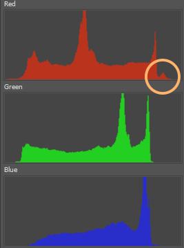
PS. Small adjustments in gain improved the histogram and high-contrast image.

$ libcamera-still --awb=daylight --tuning-file=‘imx477_scientific.json’ --saturation=1 --awbgains=1.58,1.86 --denoise=off --rawfull=1 --mode=4056:3040:12:P --encoding png --raw --n --shutter=1000 --o filename.png

[cpixip]

@PM490 - a question. I noticed while scanning Kodachrome film stock a slight magenta tint on burned-out image areas, like a very bright sky. In your above scan, the same is happening. While the WB is perfect for the film gate, the sky of your scan shows a slight magenta tint. Of course, nothing one could not correct in postproduction, but I wonder if this is a common “feature” of some film stock. I haven’t noticed such a tint for example on Agfa MovieChrome. Do you know the film stock of your scan example?

[PM490]

@cpixip

nothing one could not correct in postproduction

Or that the human perception would not white balance when projected.

@cpixip

Do you know the film stock of your scan example?

It is Kodachrome 83.

[cpixip]

Interesting. So it seems to be Kodachrome-specific. Here’s a scan which shows a similar magenta tint in very bright image areas - note that the sprockethole is more or less “white”, whereas the burned-out areas of the man’s shirt have a slight magenta/redish tint.

[PM490]

Interesting, I had not noticed it. When I start scanning with the new setup (not anytime soon), will keep an eye for it.

In looking at the markings, I also learned that Kodachrome has the fabrication and development markings . I did not know about the later, and it includes the year and month of processing.

This one is very prominent, but in other rolls is smaller and barely visible, but it is there.

[PM490]

Another testing of the sphere output port, round cropping to avoid the edges.

The difference between the magenta-low and the white-high is about 10 units in a 8 bit/ channel png.
The camera is not perfectly aligned with the center axis of the output port, which may be part of the difference between the high-white spots. The low-magenta spot corresponds nicely with the location of the PCB that is currently off, hence, the magenta-lows should even-out with the highs of the other white spots once the third port is on.

The intent of the wide output port-to sphere diameter is not to be used edge-to-edge for a final capture, but rather to take have the option of capturing a larger portion of the prior and next frames. The test shows that a 40mm port on a 100mm diameter sphere is bordering the hot spots of the entry-ports and has a substantially flat center-production area.

[npiegdon]

@cpixip

Here’s a scan which shows a similar magenta tint in very bright image areas…

That’s an interesting image. I just tinkered with it for a bit in Photoshop and it seems like the part that makes it a little more challenging for automatic color correction is this little extra bump at the high end of the red channel:

That seems to correspond to the bright red shirt belonging to the person sitting on the ground. When you run Photoshop’s “Auto Tone” algorithm, it doesn’t want to throw that information away, so it remains in the now-stretched-out extents of the histogram channels. The result is even less realistic color where everything is too cyan and the skin/hair tones (along with the pillars) all look wrong:

But if you then manually clip that little bump out of the red channel (using the “Levels” tool), both the original magenta cast and the new cyan cast are fixed:

Skin/hair/pillars all look natural, the blown out shirt is whiter and everything is looking pretty good. Even the bright red shirt hasn’t materially changed.

It almost feels like that little red bump in the histogram is a kind of “out of gamut” color that the sensor is picking up but that our vision system would have naturally “clipped”. I’ll also keep an eye out for this once I start scanning Kodachrome material.

[d_fens]

hi,

I don’t want to post all over the place, and guess this fits here best: testing the flatness of the light.
After setting the white balance this gray image is the result:

this is unedited and show some aperture-shaped dots which don’t move when moving light,rotating the lens and rotating the hq cam so i guess this must sit on the sensor? i can’t see anything on it and i’m out of ideas

The question is:
how would you rate this result and are there any improvments that can be made to remove the spots

additionaly i ran this through the Surface plot to get a better visualization

[Manuel_Angel]

Hi @d_fens,

For your peace of mind I can tell you that the image from my sensor is almost exactly the same. A neutral medium gray practically uniform over the entire surface, but yes, with several spots.

When I bought the camera, I treated it with the utmost care to avoid the deposit of dust particles on the sensor.

I removed the cap and immediately, with the sensor facing downwards, mounted the lens with the extension tubes and adapters. I have never disassembled it again and yet the stains appeared.

I cannot upload an image for you to compare, now I am not at my usual address where I have my device.

However, I think there is no cause for concern. In real catches these undesirable spots are not noticeable.

Regards

[PM490]

@d_fens

aperture-shaped dots which don’t move when moving light,rotating the lens and rotating the hq cam so i guess this must sit on the sensor? i can’t see anything on it and i’m out of ideas

I have similar dots. Went as far as to illuminate the sensor without lens, and these still there.

@PM490

To exaggerate these, with imagej one can use the Process/Enhance Contrast, with 0% saturated pixels, and the gray picture better show the issues. In the picture you posted, it shows some of the spots are pentagons (iris of the lens), and some are significantly smaller, which could be dust spots on the sensor (or IR filter in the sensor). Using the enhance contrast will also show any slight deviations of the white balance. Recommend you save the image in a format without compression, otherwise you will see a lot of the compression artifacts when doing the enhancement.

In the images above, I also set denoise to off, reason why the noise may seem a bit higher.

@d_fens

The question is:
how would you rate this result and are there any improvments that can be made to remove the spots

additionaly i ran this through the Surface plot to get a better visualization

The surface plot looks flat, if that is with the lens at the focus distance, you have great results. Try the enhance and see if it will give you additional clues to chase the spots.

[PM490]

Continuing with the SnailScan project, here is a quick status report.

One of the recurrent items in the forum, is the control of light/LEDs. I previously posted a constant current design that I used on the projector-parts based scanner. The old design used a PWM control signal, which was converted to a DC voltage, and change the LED current. For clarity: the LED current was constant, not PWM. The conversion from PWM to DC uses a filter, which introduces a reaction time. The better and more stable the DC, the longer the reaction to change current at the LEDs. A trade off to use a simple control line, which as the original posting mentions, takes advantages of workarounds to have 16 bit control. For the application, it was manageable, but there was certainly room for improvement.

The protoboard of the electronics for the new build, consist of:

• Raspberry Pico
• Three TMC Stepper Drivers (supply, pickup, and capstan).
• I2C DAC (8 outputs, 16 bit each)
• DAC to LED Driver Buffer (only one).
• Voltage regulators.
• The sphere with 3 LED Boards, each Board has 4 LEDs, each LED runs at 3/4W max (for about 9W max total).

The black PCB is the old driver, used in the proto-boarding for the current mirror transistors and the voltage regulator.

This is the schematic of the improved LED driver.

The gray box are shared components with the old design. Whatever current is set at Q3, will be mirrored by Q4, Q5, Q6, and Q7. If Q3 is sensing 75 mA, the four transistor in the mirror configuration will total 300mA.

Using the same configuration, I would like to share some of the improvements.

Two Supplies
The new design uses two voltage sources VL = 15V, and VLED = 32V (these LEDs have a Vf of 9V, so having a cascade of 3 requires voltage higher than 27V and must include headroom for the transistor Vce).

Being a linear design, the various configurations and specifications of LED require different voltages for the LEDs. But the driver does not have to be linked to that higher voltage, since the interface with the drivers is current driven.

It makes everything cooler, since the parallel resistors can be driven by the same current, but with a lower voltage… less heat.

DAC to Mirror
In the old design, the base of the darlington-pair was driven by the DC generated by low-pass filtering the PWM.

In the new design, instead, an OpAmp configured as non-inverter amplifier, and buffered by the same darlington-pair prior, now takes the DC output of the DAC (0 to 5 V) and conditions it to the desired current level needed at the current mirror.

Flexibility
This configuration can be adapted to different ranges in DAC, different LED voltage requirements, and different currents, only by changing values of resistors.
The same board can be used for widely different LED requirements too, from the extreme represented above (large Vf with large current).

Repeatability
A board for the components of the schematic, times the number of colors (up to 8 for the DAC), and one can put together a multi-spectrum-stop-motion scanner. This part is solved.

Limitations
Because of heat management at the LEDs inside the sphere, this is not intended to work continuously-on while at full intensity. Also it is likely that all the available light will not be necessary, it is a bit of an overkill, but I am taking advantage of the prior design/components. Reducing the light output during the movement period is sufficient to cool it off.

Next steps
Light is the one item of the scanner that I have dedicated the most time, and iterations. I am pleased with bringing it to this level, and hope that sharing these findings help everyone in their journey.

Note: experience is what you get, when you don’t get what you want!

No amount or ability to control light can make the film move! My next challenge is to assemble a new transport with the experience of the earlier failures.

Coming up…

• The transport design is getting there, and I hope to send the parts out for laser-cutting in the next few weeks.
• Two PCBs will be designed to assemble the electronics. The PICO, 8-channel DAC, 3-stepper drivers, in one. The LED Driver only (schematic above) will be the second PCB.
• Testing the assembled components (transport and electronics).
• Finalizing programming of the PICO to receive USB-Serial commands for the transport/light control.

[npiegdon]

This is a nice update. That new LED control circuit looks very flexible! I’ll agree that it does seem a bit over-powered. I’ll be curious how much of that light you end up using. In the same size integrating sphere, my ~2W lights already lead to rather short exposure times. That said, too much light is a better problem to have than too little light…

@PM490

No amount or ability to control light can make the film move! My next challenge is to assemble a new transport with the experience of the earlier failures .

Reading through your older post, you described what the ToF sensor was attempting to do, but I’m not sure I understood why you needed an accurate spool diameter. Were you planning to essentially “fly blind” and use only the spool diameter to calculate how far to advance to the next frame? You weren’t planning to use a computer-vision based approach (say, like the one cpixip has described in a couple places)?

I’d thought about going in the other direction: using a vision-based approach to advance frames, which then gives you a spool diameter-like metric for free. Each frame, the direct-drive steppers will each move a little differently. The take-up stepper will move a little less and the supply stepper will move a little more. If you keep track of the number of steps it takes to advance each frame, it shouldn’t be hard to fit a curve and get a rough metric for how much film is left on a spool. You may need an estimate of the core diameter to get any real accuracy here, but it seemed like a nice way to get a kind of free metric that could be used to display an overall progress bar for the reel.

To use the diameter as a data source for driving the frame advance seems like it’d be tricky. Even with all the accuracy you could ever hope for, all the other confounding variables (different film stock thicknesses, the presence of an audio track, any sort of debris, shrinkage/warping, or even the tightness of the wind) would make it a nightmare to pin down, wouldn’t it?

[d_fens]

@PM490

Try the enhance and see if it will give you additional clues to chase the spots.

i followed your advice and captured the uncompressed sample, enhanced it and have mixed emotions:

While the flatness looks good to me, the “cleaning” just added new dirt, back to square one, rinse and repeat …

Interesting read about your lighting endeavors, i’ve settled for three Cree white LEDs and a Meanwell driver, but I can’t use the PWM dimmer feature as its frequency is maximal 1KHz which produces lines artifacts with those short exposure times and I dropped the idea of controlling the light vs controlling exposure time. Still i might get rid of the fan when switching them off during transport.

[PM490]

@d_fens

While the flatness looks good to me, the “cleaning” just added new dirt, back to square one, rinse and repeat …

@d_fens flatness looks excellent. I have not been able to take out every spot, but the high contrast was useful in locating the small dark ones, typically does are dust on the sensor. Great progress.

[PM490]

Thanks @npiegdon

@npiegdon

Reading through your older post, you described what the ToF sensor was attempting to do, but I’m not sure I understood why you needed an accurate spool diameter. Were you planning to essentially “fly blind” and use only the spool diameter to calculate how far to advance to the next frame? You weren’t planning to use a computer-vision based approach (say, like the one cpixip has described in a couple places)?

I’d thought about going in the other direction: using a vision-based approach to advance frames, which then gives you a spool diameter-like metric for free.

The build uses geared stepper motors directly to the reels, with incredible precision to supply/take up film. The problem is that the diameter of the spool determines the steps that each (supply/take up) require to move one frame. Film thickness is included in the spool diameter.

One of the goals is to be able to digitize Develocorder films, basically 16mm films without any perforation or frame. Computer vision is possible, but not as straight forward as detecting the perforation. It would involve either using the image displacement to measure the advance, or reading the time code track.

The idea was to use the math of turning a variable diameter spool. And the math actually worked pretty well, as I tested after giving up on the ToF. In that case, it required to include the film thickness in the calculations, and to my surprise, the results were better than expected. I think this is what you referred as flying blind, and it would not be practical, specially since warped film can change the thickness along the length of the reel.

The bottom line is that ToF sensors did not have the resolution (these measure in 1mm increments), nor accuracy. In ideal conditions, when used against the film at the spool, these would be all over the place. Accuracy improved somewhat against a while target, but it wasn’t ideal.

It was great experience, and it helped test other components, like the tension sensor. And it was also interesting to fly it blind (no sensors, only setting the spool diameters and film thickness at the start), and see how well it performed.

@npiegdon

I’ll be curious how much of that light you end up using. In the same size integrating sphere, my ~2W lights already lead to rather short exposure times. That said, too much light is a better problem to have than too little light…

Agree. It is definitely an overkill.

I do have one film that was poorly developed and is extremely dark. On the first scanner I was able to get the content but with very poor quality (even with very long exposures, the image content was minimal). It will be a good test case for the extra light.

[Manuel_Angel]

@d_fens,

I have obtained this image with my device under the same conditions.

Very good observation by @PM490. What to me were simply “spots”, in effect I have observed that they have a pentagonal shape, in correspondence with the iris of the five-blade diaphragm of the Rodenstock Rodagon 50mm f 1:2.8 lens.

What I fail to understand is why they appear in seemingly random places.

[d_fens]

@PM490

The bottom line is that ToF sensors did not have the resolution (these measure in 1mm increments), nor accuracy.

I’ve been thinking about a method to precisely transport non-perforated film, the idea revolves around the use of two big wheels pressing from above and below onto the film. These wheels would have a rubberized surface to prevent the film from slipping.

To ensure precise positioning, one could construct a series of holes into one of the wheels. A light barrier (or sensor) would then be used to detect these holes as they pass, allowing the system to halt at the next hole. This should, in theory, allow for frame-accurate transportation of the film.

I’m curious to hear your thoughts on this. Does this seem like a viable solution? I know it’s not as elegant a some don’t like the idea of touching the surface.

Another approach would be training an AI model with suitable datasets as a standalone solution, but therefore a fast model with realtime detection should be used

@Manuel_Angel

What I fail to understand is why they appear in seemingly random places.

This sounds like dust on the objective, does it move when you rotate the objective?

[PM490]

@d_fens

I’ve been thinking about a method to precisely transport non-perforated film, the idea revolves around the use of two big wheels pressing from above and below onto the film. These wheels would have a rubberized surface to prevent the film from slipping.

One example of something like it is Denis Carl’s main drive in the Gugusse Roller build.

@d_fens

I’m curious to hear your thoughts on this. Does this seem like a viable solution? I know it’s not as elegant a some don’t like the idea of touching the surface.

The new transport will test a U-Capstan, where the film is pressed to the capstan by tension, instead of another roller pressure directly. This part is yet untested, it will be assembled with the laser-cut plates. Here how that portion looks.

The silicone roller (yellow) is driven directly by a geared stepper motor, the two reels are also mounted on the axis of geared stepper motors. I found a silicone wheel that is 10 mm height and 50 mm diameter, so the precision is there to move the film very accurately, as long as the film holds to the roller (the testing part). The Zs in the path are the tension potentiometers, when the film is in tension there will be no Zs in the path. The bottom reel is the supply, the top reel is the pickup.
The capstan will increase the tension at the supply side, and decrease the tension on the pickup side.
The tension sensors on either side will provide the feedback/control to unroll the supply side to hold the tension from increasing, and roll the pickup side to hold the tension from decreasing.
In the previous run, I tested the dancing potentiometer tension sensor.

20221106 Scanner - Tension Arm Proof of Concept

It worked well with very rudimentary software. The new one is a 3D printed hat to hold the conic posts, the circles on the Zs.

[justin]

Has anyone looked into applying a flat field correction? I have used it when DSLR scanning 35mm slides via my raw processor Capture One.

An example of flat field correction with Lightroom

A quick Google search didn’t reveal any function already available in open-cv.

I feel like I’ve read about a similar method for minimizing dust errors, but I couldn’t find anything. I need to do a better job of bookmarking.

[PM490]

@justin I haven’t explored flat field, but it sounds like an interesting option to consider.

Back to SnailScan, small progress to report…

@PM490

This is the schematic of the improved LED driver.

This is what the first Kicad sit-down PCB board looks like for the new LED driver design, 110mm x 30mm (no traces yet).

Prior I mentioned that the design would be two Boards. Instead, now working on a third board configuration. The DAC, its voltage regulators, and a DAC bus, will be a separate board.
It will reduce wiring… DAC will have a connector BUS for all the drivers boards, where up to 8 can be connected at once (one per each DAC output).

This change was done to minimize the area of the PCBs, now opting to stack the Drivers with the DAC board as bus/backplane.

A nice byproduct is that it would make the DAC and Drivers virtually stand alone to work with other controllers with an I2C master, like other development boards, or the RPi.

The Pico will stay with the stepper drivers, and will now have a I2C connector to drive the stand alone DAC/Driver block.